Consistent within the checks
The model passes the tests that were applied. Other explanations may still be possible.

Press Play to watch the Sun change. The original shows the supplied image. A base difference compares it with the first frame; a running difference compares it with an earlier frame. In the difference panels, white means increased brightness and black means decreased brightness. Use the Frame slider to look at one moment.
All 51 frames are included. Opening and reopening start at frame 23.
Event association: 10 September 2017, from the supplied description. Source: JPEG frames from the developer’s local archive. Instrument attribution: GOES/SUVI; exact archive matching, passband and observing times remain unverified. These rendered-image changes help locate features; they do not establish a density jump or a shock type.
13 June 2010 · SDO/AIA science team. Frame processing and crest marks: RMO (R120). Motion in images alone does not determine the MHD type.
These are the actual SDO/AIA 193 Å images. Teal marks the inner ridge; orange marks the outer ridge. The colors do not assign fast or slow.
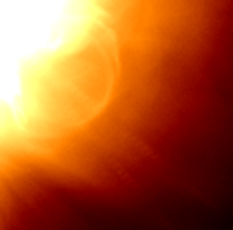
SDO/AIA · 13 June 2010 · exposure-normalized data
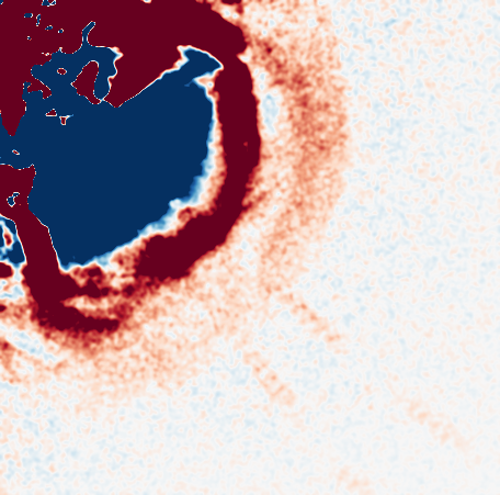
Red: brighter; blue: dimmer. Fixed scale ±12 DN/s.
Solar X: 850–1214 arcsec; Solar Y: −710 to −350 arcsec. Actual exposure times are shown; playback is for inspection. Late low-contrast candidates carry no accepted overlay. Turn the fits off to inspect the images themselves.
Every view uses retained pointing updates and exposure normalization. The display alone is smoothed with a Gaussian sigma of 1.2 arcsec. The original uses a fixed asinh stretch (width 20 DN/s, limits 0–800 DN/s). The base views use fixed limits ±12 DN/s; running differences use ±4 DN/s. Clipping and different display scales prevent a direct comparison of panel colors as amplitudes.
Reference A is 05:35:08.07 UTC; B is 05:36:08.09 UTC. Running differences subtract the previous consecutive science image, about 12 seconds earlier. No temporal smoothing or interpolation. The first science exposure has no running panel because its preceding retained frame is two minutes earlier.
Overlays use the same quadratic fit to ridge samples over PA 116° ±1° as the central geometry calculation. Weak outer crests have less regular raw samples. The full samples, windows, method failures, original FITS names and hashes are saved with the result. The images support a motion measurement; they do not measure plasma flow, density or field.
A bright front moves across the Sun. What is the plasma doing?
RMO helps you compare possible explanations, see what has been checked, and find which measurement is missing. Start with a ready-made example; you do not need to enter numbers.
Ready-made results, figures and explanations work in this HTML. A fresh numerical diagnosis requires the compatible Python calculation service; its connection status is shown with the controls.
Begin with the sentence above the figure. Then ask what inputs it used and what alternatives were actually checked.
The model passes the tests that were applied. Other explanations may still be possible.
Those inputs do not pass that check. Read which condition failed; a numerical failure alone does not identify a different physical process.
An input is missing, errors leave alternatives open, or the method does not cover this case. This is a useful result: it tells us what to examine next.
“Uniquely identified” requires more: the relevant competing explanations must be excluded using adequate observations. A fast label on a model alone does not do that.
Two words you will meet: plasma is the electrically conducting gas; MHD describes its motion together with the magnetic field. “Fast” and “slow” name wave families relative to local characteristic speeds, not simply a fast or slow feature on an image.
Which errors can the result tolerate? Read the tested input errors, whether the conclusion survives them and, when established, the limit of the stated criterion. Input uncertainty is distinct from a solver residual or model limitations.
How to read an error: the central value comes with ± an amount or ± a percentage; unequal bounds use −lower/+upper. Read the units and whether the limits are hard bounds or statistical errors. Labels 1σ, 2σ and 3σ require a stated statistical meaning; hard bounds are not converted into sigma. Individual error bars also do not specify which combinations are allowed.
Saved results: what RMO has established and the next observational test. Angle and speed errors. Earlier figures and tests remain in the MHD section.
R132 · E05 · calculation complete
Both conditional fast and slow families survive. Front-normal tilt is the useful discriminator in the tested planning cases. A tilt of 45° ± 5° excludes the checked slow family; 60° ± 5° excludes the checked fast family, with θ allowed over all 1–89°.
The final continuous exclusion includes unresolved portions of those strips. Field angle alone does not discriminate at the checked 30° and 80° cases. These are conditional planning bounds, not measured front angles or observed E05 mode identifications.
R132 records the geometry-discrimination calculation. Subsequent observational checks are available in R133–R139 below.
The saved scientific evidence distinguishes measured quantities, source-derived reductions, assumptions and model results.
| Category | Fixed R131 quantity / interpretation |
|---|---|
| MEASURED | Relative centroid +16.559600881163973 km/s; emission-weighted relative redshift, not a directly measured state jump. |
| SOURCE_DERIVED | Conditional effective density 235053642.40666732 cm⁻³ from saved R130 spectral reduction. |
| SOURCE_DERIVED | Published EIS surface-speed proxy 371 km/s, credited to Veronig et al. (2011) in retained R131 provenance. |
| ASSUMED | Density assigned downstream; reference treated as upstream; centroid assigned to the model jump; upstream rest; T₂ = 1584893.1924611141 K. |
| ASSUMED | Ideal planar isotropic MHD, γ = 5/3; ionized hydrogen; Tₑ = Tₚ; no added heat flux; fixed registration, zero height and northward surface tangent. |
| ASSUMED / SCANNED | Downward normal tilt α and upstream field-to-normal angle θ. Field/velocity tangential azimuth remains fixed by e₁ ∥ n × LOS and zero e₂ velocity. |
| MODEL_DERIVED | Normal speed D, μ, compression X, upstream thermodynamic state, fields and velocity jumps. Recomputed from the same constraints; never independently tuned. |
The aperture remains central rows 334–338, exposure 25 and reference exposures 1–10. No spectra were refitted, no temperature/reference was retuned, and no R0–R131 calculation was repeated. Published observations, atomic data and external software retain their existing source credits. R132 adds a conditional model map and the precision exclusion proof.
The normal is tilted downward from the fixed local surface tangent t toward −r. The LOS unit vector ℓ points toward the observer. Positive d is the saved relative redshift.
The saved normalized velocities are v₁/D = [0, 0, 0] and v₂/D = [1 − 1/X, −bₙ(bₜ₂ − bₜ₁), 0]. Therefore the dimensional tangential vectors are vₜ₁ = 0 and vₜ₂ = −D bₙ(bₜ₂ − bₜ₁)e₁, with e₁ = (n × ℓ)/|n × ℓ|.
The tangential LOS projection follows from this velocity construction. Both state vectors and their difference were explicitly checked at every accepted root. Maximum relative residual: 1.3221 × 10⁻¹⁸, below 10⁻¹². This geometry remains ASSUMED; it is not an observational finding inferred merely from Bₜ.
The scan covers α = −89–89° and θ = 1–89°, initially at 1°, with adaptive spacings 0.5°, 0.25° and 0.125° and a 50,000-location cap. There are 41,028 saved angular locations. The final lock performs continuous interval evaluation of a necessary sign, not a further MHD root sweep.
The energy equation is quadratic in z away from the guarded rational pole. All algebraic roots, including complex/negative/rejected candidates, are recorded. There is no finite field-strength cutoff. Stable quadratic arithmetic and 70-digit Decimal fallback near cancellation do not override the numerical guards.
| Predeclared numerical threshold | Value |
|---|---|
| min_abs_mu | 0.001 |
| min_cross_norm | 1e-08 |
| min_compression_denominator_margin | 1e-06 |
| min_compression_excess | 5e-08 |
| min_pole_relative_distance | 1e-06 |
| polynomial_root_residual | 1e-12 |
| flux_residual | 1e-10 |
| min_relative_leading_coefficient | 1e-12 |
| min_relative_discriminant | 1e-12 |
| min_relative_root_separation | 1e-07 |
| characteristic_guard | 1e-07 |
| field_component_guard | 1e-08 |
| entropy_guard | 1e-09 |
| pressure_guard | 1e-10 |
| tangential_LOS_relative | 1e-12 |
| Doppler_absolute_km_s | 1e-09 |
Pole distance is |1 − Xbₙ²|/max(1, |Xbₙ²|). Polynomial residual divides |az² + bz + c| by |a|z² + |b|z + |c|. Characteristic margins are scaled by max(1, all normalized flow and characteristic speeds); the same guard applies to characteristic coincidences. Full definitions are in the frozen specification. None of these thresholds changed after seeing the map.
Each accepted root passes positive pressure, compression, increasing entropy, conservation and the ordinary characteristic transition: 1 → 2 for fast; 3 → 4 for slow. The unchanged R131 diagnostic and an independent dimensional flux check agree. The maximum accepted independent scaled flux residual is 1.1022 × 10⁻¹², below 10⁻¹⁰.
| Map-node status | Count |
|---|---|
| FAST_ONLY | 10769 |
| SLOW_ONLY | 3816 |
| BOTH | 0 |
| NEITHER | 25725 |
| UNRESOLVED | 718 |
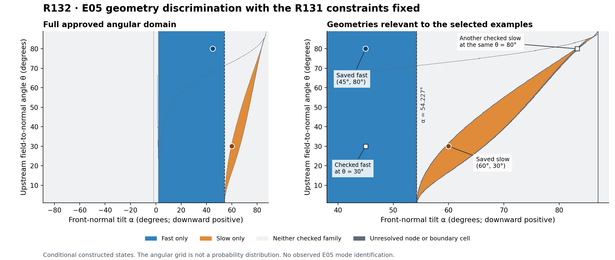
There are 52,110 algebraic root records and 15,151 accepted ordinary roots: 10,769 fast and 4,382 slow. At 555 angular locations two accepted slow roots survive. They are retained as alternatives, not ranked as probabilities. At (83.25°, 80°), two checked slow roots have upstream fields about 1.35332 G and 3.07095 G.
The 718 unresolved nodes include 705 small-|μ| guard locations and 13 characteristic-degeneracy locations; 11 of those 13 also retain an accepted slow root, without changing the unresolved node label. There are 8,462 unresolved boundary cells at the final 0.125° spacing. Changes in rejected-root status can also create gray cell boundaries. Adaptive counts are not area fractions or probabilities.
For an ordinary checked fast transition, bₙ² < 1/X. The bracket in H then exceeds (X − 1)(5X − 2)/X > 0, so a positive finite root requires A < 0. For an ordinary checked slow transition, bₙ² > 1. The bracket is then less than 3(1 − X) < 0, so a positive finite root requires A > 0. This excludes the two ordinary families at the same geometry within this closure. It is not general MHD uniqueness.
A depends on α alone for the fixed inputs. Its valid positive-tilt zeros are approximately 2.121854° and 54.226970°. A is negative between them and positive above the upper zero. The lower positive-A region does not by itself establish a slow solution. The separator near 54.227° is a conditional model result, not a measured front angle.
| Planning strip | Full θ range | Continuous A enclosure, rounded outward | Intersecting unresolved boundary cells | Excluded ordinary family |
|---|---|---|---|---|
| α = 40–50° | 1–89° | −2.475 < A < −0.807 | 110 | slow |
| α = 55–65° | 1–89° | 0.00608 < A < 5.844 | 779 | fast |
Final lock: PASS. Sixty-digit outward-rounded interval arithmetic covers contiguous 0.125° tilt intervals throughout both strips. The evaluation includes conservative numerical padding of fixed inputs, not added observational uncertainty. The necessary sign excludes any hidden competing ordinary root for all θ = 1–89°, including inside the listed unresolved boundary cells. Guarded states and cells are not relabelled. No conclusion downgrade was needed.
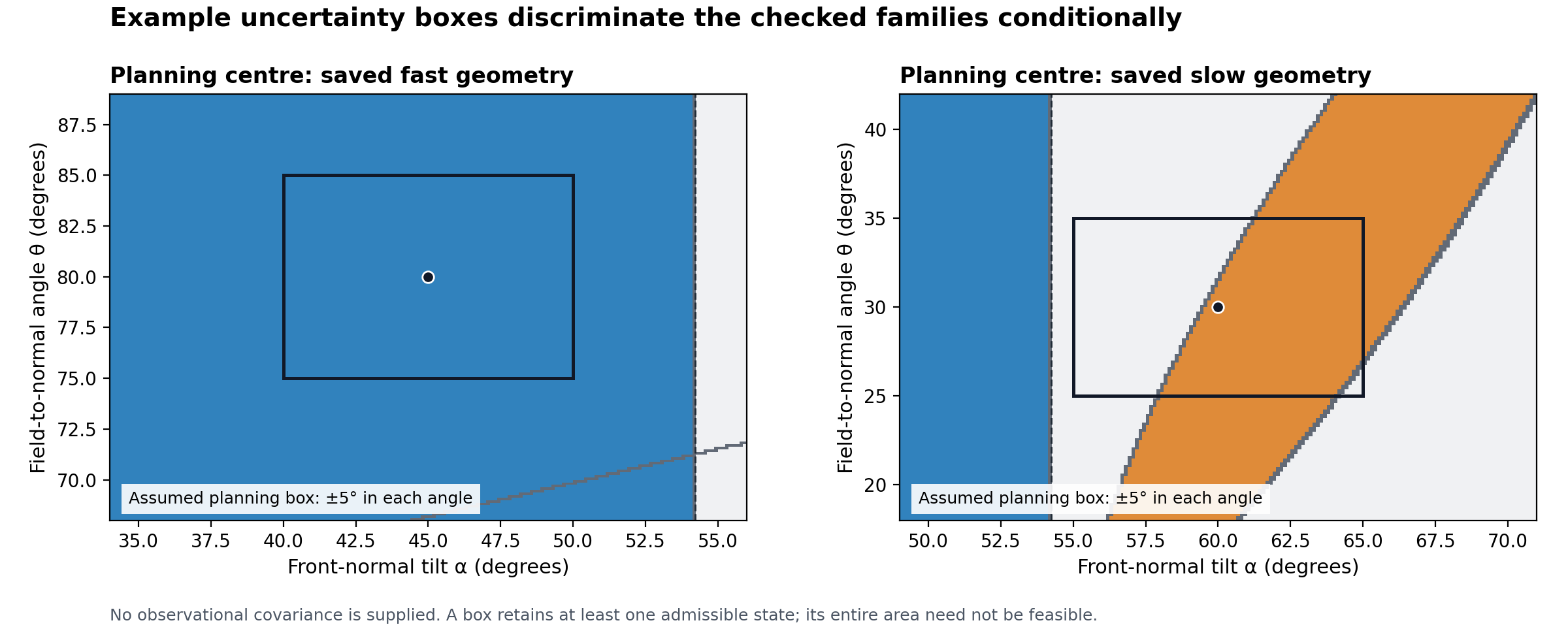
The planning region is an ASSUMED axis-aligned [α₀ − δα, α₀ + δα] × [θ₀ − δθ, θ₀ + δθ] box. No covariance ellipse or confidence level has been measured. A discriminating box retains at least one admissible state and excludes the competing checked ordinary family; not every point in it must be feasible.
45° ± 5° excludes checked slow; 60° ± 5° excludes checked fast, with the other angle allowed over its full tested range. These are sufficient conditional planning bounds near selected centres. They are not universal observational uncertainties and do not come from simply subtracting the two example angles.
Field angle alone is insufficient even at zero error in the checked cases: fast (45°, 30°) and slow (60°, 30°) share θ = 30°; fast (45°, 80°) and slow (83.25°, 80°) share θ = 80°. The saved (45°, 30°) fast state passes conservation, entropy and the 1 → 2 transition with independent residual 7.27 × 10⁻¹⁶. It is not a label-only scenario.
Measured and source-derived input uncertainties were not propagated in this geometry-only calculation. Field azimuth, upstream rest, thermal closure, front association and registration remain assumptions. The finite map does not certify every continuous cell interior or exclude all thin unsampled branches. The final sign proof certifies only the specified competing-family exclusions. “Neither” does not exclude every MHD solution, full fan, smooth-wave interpretation or observational alternative.
These are known model cases with exact inputs. No type label was supplied to the diagnostic. Separate conservation-law and characteristic-speed calculations agreed. In one further model case, compression and normal acoustic Mach exclude fast without magnetic inputs; removing flow or thermal information admits constructed fast alternatives. The exclusion also survives two declared hard-bound sets; a wider Cartesian set admits a newly checked fast state as well as the saved slow reference, at different complete states. For central normal Alfvén speed cAn,₁ = w₀, hard errors of ±20% preserve fast exclusion, with a limiting symmetric error of about ±24.4% for this criterion; these are not 1σ errors. Compression ±0.05 and normal acoustic Mach ±10% are already included. These constraints are imposed model inputs, not inferred from observations. These are model results, not four solar identifications.
R132 — preservation and reproduction
The original executed scripts in code/, frozen specification, saved numerical outputs and review records are retained exactly from the approved calculation. code/final_scientific_lock.py supplies the additional continuous sign verification. It does not run a new MHD sensitivity sweep.
reproduction_code/ contains the same four calculation scripts with one portability change: r132_model.py obtains the R131 baseline directory from the environment variable RMO_R131_BASELINE. No equation, threshold, root-selection rule or physical criterion was changed. The run-time source hashes in earlier records refer to the executed snapshot; BUNDLE_MANIFEST_R132.json hashes the delivered copies.
For numerical reproduction, use a separate empty output directory and the supplied reproduction scripts. Preserve the frozen input specification and compare physical values with the declared residual and conditioning criteria. See the reproducibility instructions for required source records and dependencies.
A fresh run may differ in timestamps, cached-node ordering, gzip metadata and execution-time hashes. Scientific reproduction compares states by (α, θ, root) and uses the declared residual/conditioning criteria. Exact transport reconstruction, in contrast, compares every delivered project file by path, byte count and SHA-256 and requires exact agreement.
The final scientific lock can be checked with code/final_scientific_lock.py --review PATH_TO_REVIEW_LAYOUT --output NEW_EXTERNAL_OUTPUT.json. That layout must provide the saved code and results; the original snapshot expects the original baseline path, while a temporary copy may use the documented portable r132_model.py. The lock uses only interval evaluation of the necessary sign condition and reads the saved angular results. Do not overwrite the saved lock output.
Complete CSV/JSONL root records, PNG/SVG/PDF figures, code and manifests are supplied separately and inside the incremental update. Earlier REVIEW strings in retained records are historical; the final scientific lock and final checkpoint manifest establish R132 status.
Choose a model to see its front type, speed plot and physical checks.
What are we analysing? Two neighbouring plasma regions separated by one moving front. We compare their density, pressure, plasma motion and magnetic field to identify the type of front under the stated MHD assumptions.
This is a model demonstration: the parameters are artificial and fully specified. Start with a saved example to see the method work. For measured solar motion, use the real EUV example. The names fast and slow refer to MHD wave families.
Follow the result: read the one-sentence answer, look at the speed plot, then open the physical checks if you want the details.
See the result, speed diagram and physical checks. This is a constructed model, not a solar observation.
Load the checked perpendicular model, then choose the error range. RMO applies the current physical checks automatically.
RMO checks whether the same front type remains supported when the inputs vary within their stated error ranges, while respecting the physical relations between the states.
Conservation laws link the true plasma states on the two sides. Errors in separate measurements may still be independent. Keep the measured values and their uncertainties: RMO does not change them to obtain a preferred answer.
For this perpendicular model, the magnetic field lies along the front surface: B_n and its error width are fixed at zero. The type statement applies to conservation-compatible states within the supplied ranges, under the single-front ideal-MHD assumptions. Uncertainty in the field angle is not tested by this example.
The input-bound factor scales the stored error widths. It is not a confidence level or the same percentage for every field. Open Parameters and input file to see the actual ranges. The result, speed plot and physical checks below refer to the current method.
The exact central model was checked separately using conservation laws and characteristic speeds. Those checks remain part of the result. An inconsistent central input is not silently repaired.
Choose a model and click Load checked example. No parameters have been loaded here.
Record what is known for one front patch and time. Missing quantities may be represented by justified literature scenarios. Keep their origin and error meaning visible.
Source: Table 1, printed p.108 (PDF page 114 in the supplied book). 1 T = 10⁴ G; 1 m⁻³ = 10⁻⁶ cm⁻³.
These are typical averages. Choose and justify scenario widths separately; the table does not provide ± errors. It does not provide a magnetic direction or a front normal. Its nH column means neutral hydrogen, not the ion density.
The prominence and chromospheric rows require additional ionization/coupling assumptions and are not offered as automatic coronal presets. Table 2 gives scale estimates; derive pressure, mass density, Alfvén speed, sound speed and beta consistently from the adopted physical state.
Units: this worksheet uses physical units. The numerical model editor below uses normalized units. A temperature and electron density do not by themselves specify total pressure and mass density; record composition and electron/ion assumptions. Field magnitude does not specify its vector.
“From this event’s data” may include an observation-based diagnostic; record its method and assumptions. “Published estimate” refers to this event. A typical value for another coronal structure stays ASSUMED. The table buttons preserve entries marked as event measurements or published event estimates.
Unknown inputs remain blank. This is a preparation worksheet; it does not run a shock diagnosis.
Level A: aim to recover as many constraints as possible from the event data. Level B: combine event constraints with stated literature scenarios. Level C: explore which future measurements could distinguish alternatives. These describe evidence coverage, not the wave family.
A conclusion is robust under declared literature-bounded assumptions only if the applicable test covers the full allowed joint set. A finite grid supports a statement about the sampled cases. Failure to exclude fast does not prove an admissible fast state, and fast exclusion does not uniquely identify slow.
Every observational result must carry this provenance table. For an angle, distinguish a measured projection, a reconstructed three-dimensional angle and an assumed orientation. A geometric reconstruction inherits its input assumptions and needs an uncertainty explanation. A model-predicted downstream temperature is not an independent measured check of the same model.
The illustrative intervals 5–15 G and 3–20 G, and the 12 G threshold previously considered, are not results of RMO and are not defaults here.
Normalized model units, mu0 = 1. LEFT and RIGHT are the adjacent states of this one discontinuity in a common local frame. They are not the remote initial states of a full wave fan. The flow direction determines which side is upstream.
Enter a central value and an absolute half-width: value ± half-width. Blank means unknown; it is never zero. Gamma and the normal direction are fixed assumptions in this test. The preset factor uses f |value| for density/pressure and f max(1, |value|) for speeds and fields. These are illustrative ranges, not instrument errors or confidence levels.
| Quantity | Central value | Absolute half-width |
|---|---|---|
This input format is specific to local diagnosis. The older literature drafts and full Riemann requests have their own import controls below.
A new calculation requires a Python connection. Saved examples can be opened without it.
Checking whether this page was served with a Python connection.
Exact equalities are sensitive to measurement errors. The type may still remain identifiable within the error bounds. A failed sufficient test means “not certified”; it does not prove that two physical branches remain possible.
It compares plasma motion relative to the front with the slow, Alfvén and fast wave speeds on each side. Their ordering helps identify the front type. Each bar spans the range allowed by the chosen input bounds.
Speed intervals and strict inequalities apply to a single conservation-compatible planar ideal-MHD discontinuity. They do not establish full Riemann-fan uniqueness or identify an EUV image feature.
FAQ: how do measurement errors affect the result?
Four known test fixtures, with reference labels kept outside the diagnostic input. Fast and slow inequalities survive some finite bounds; contact and rotation require an uncertainty model that respects their equalities.

Save the complete study figure · vector PDF
# RMO-75: input errors and local MHD diagnosis

## Result in one sentence

The two synthetic shock types remain conditionally identifiable for some finite
input bounds, although noisy central values fail the tight exact-conservation check.
These are model demonstrations, not classifications of solar observations.

## What was found

- Fast shock A63 passes the sufficient interval certificate at factors 0.01 and 0.05.
- Slow shock A17 passes at 0.01. At 0.05, entropy and the downstream slow-speed crossing are not certified.
- At 0.10 neither shock passes the initial sufficient test; this is not evidence for a second feasible solution.
- At 0.10 for A63, tightening only pressure half-widths to 1% restores the certificate. This demonstrates a useful additional constraint, not a globally optimal observing strategy.
- Exact contact and rotational-discontinuity diagnoses are retained. Their equality constraints are not certified by a free, independently varied error box.
- Missing field, front speed or pressure produces an explicit missing-measurement result. No missing value is replaced by zero or a coronal mean.

The shared speed and field correlations required by a single front are retained.
Joint covariance inference, geometry uncertainty and dynamical stability are outside
this test. The four inputs are known test fixtures with separate historical scoring
labels, not an external unseen validation set or a measured success-rate sample.

## What the percentages mean

For density and thermal pressure, half-width = f times the absolute central value.
For each velocity/field component and front speed, half-width = f times max(1,
absolute central value), in the declared normalized units. Zero vector components
therefore have nonzero uncertainty. Factors 0.01, 0.05 and 0.10 are illustrative
bounded input designs; they are **not instrument errors, standard deviations,
confidence levels or universal accuracy requirements**. Gamma and normal geometry
are fixed. Inspect every half-width in the exported request.

## Exact equalities versus measured data

Rankine-Hugoniot conservation is tested at scaled tolerance 1e-10 for an exact
supplied pair. Measurements generally have much larger errors. Failure of that
exact-pair check does not itself exclude a shock interpretation.

In two controls the downstream-pressure centre was shifted upward by 0.25%, with
the same 1% box design. The original exact point lies within the box. A bounded
least-squares search using conservation alone found a numerical witness; no type
label or saved solution was passed to the search. Every adjustment is recorded.
Independent 70-digit lab-frame arithmetic checked each witness. The witness is
**not** a unique reconstruction, maximum-likelihood estimate or posterior sample.

| Model | Noisy-centre scaled RH | Witness independent scaled RH | Certified local type |
|---|---:|---:|---|
| A17 | 0.00191 | 9.8e-13 | slow_shock |
| A63 | 0.00147 | 1.82e-12 | fast_shock |

## Full model outcomes

| Model | Factor f | Outcome | Type |
|---|---:|---|---|
| A17 | 0 | EXACT_LOCAL_CLASS | slow_shock |
| A17 | 0.01 | CONDITIONAL_ROBUST_CLASS | slow_shock |
| A17 | 0.05 | NOT_CERTIFIED | No certified type |
| A17 | 0.1 | NOT_CERTIFIED | No certified type |
| A42 | 0 | EXACT_LOCAL_CLASS | contact |
| A42 | 0.01 | NOT_CERTIFIED | No certified type |
| A42 | 0.05 | NOT_CERTIFIED | No certified type |
| A42 | 0.1 | NOT_CERTIFIED | No certified type |
| A63 | 0 | EXACT_LOCAL_CLASS | fast_shock |
| A63 | 0.01 | CONDITIONAL_ROBUST_CLASS | fast_shock |
| A63 | 0.05 | CONDITIONAL_ROBUST_CLASS | fast_shock |
| A63 | 0.1 | NOT_CERTIFIED | No certified type |
| A88 | 0 | EXACT_LOCAL_CLASS | rotational_discontinuity |
| A88 | 0.01 | NOT_CERTIFIED | No certified type |
| A88 | 0.05 | NOT_CERTIFIED | No certified type |
| A88 | 0.1 | NOT_CERTIFIED | No certified type |

Certification combines a checked numerical anchor with outward-rounded interval
bounds for compression, entropy increase, field trend and characteristic ordering.
It is conditional on a **single conservation-compatible planar ideal-MHD
discontinuity** within the supplied box. The interval tests are sufficient, not
necessary: failing a bound is NOT CERTIFIED, not proof of ambiguity between two
constructed physical solutions. No complete Riemann-fan uniqueness is inferred.

## Existing EUV example: what geometry tells us

T. Podladchikova et al. (2019), ApJ 877, 68, Tables 4-5,
[source DOI](https://doi.org/10.3847/1538-4357/ab1b3a). Event: 13 February 2009.
The same selected front patch is used, as identified in the source record by a study author.

| Point | Apparent pattern speed (km/s) | Corrected surface pattern speed (km/s) | Reduction relative to apparent |
|---|---:|---:|---:|
| 1 | 260.83 | 207.51 | 20.44% |
| 2 | 258.62 | 208.38 | 19.43% |
| 3 | 259.05 | 205.12 | 20.82% |

Thus the already published geometry changes the inferred surface pattern speed by
about 19-21%. This is a reproducibility/application check of published values, **not
a new discovery or shock-type determination**. Local normal geometry, shock-frame
plasma velocities, co-spatial thermomagnetic states and their joint errors are absent
from these extracted tables. Pattern speed and crest-height change cannot simply be
inserted as plasma normal velocity and shock-normal speed. No assumed beta or
unreported field was substituted to manufacture a solar classification.

## Verification and interface

The study passed 74 assertions, including anonymous-input scoring,
missing/invalid input controls, fixed shared Galilean offsets and normal reversal.
Independent 80-digit arithmetic checked characteristic enclosures at
384 deterministic box points. This checks the
implementation; it is not exhaustive validation or a probabilistic accuracy claim.

QuickLook offers the saved study offline, editable local-state inputs and exports.
The added Python diagnosis action uses the existing protected local service and
preserves the exact request, result, adjustments and source hashes. It is separate
from a full Riemann solve and from the preserved Brio-Wu viewer. Native Chrome,
accessibility and public hosting acceptance remain unverified.

## Reusable result summary

Exact conservation residuals and uncertainty in MHD-family classification were
evaluated separately. For two known shock test fixtures, sufficient interval tests
preserved the local fast- and slow-shock classifications for explicitly specified
bounded perturbations. Two deliberately displaced measurement centres failed the
tight exact-state conservation test, while independently checked numerical witnesses
within their bounds retained the same conditional type certificates. These results
show why failure of an exact equality test should not be identified with physical
exclusion. The certificates assume a single planar ideal-MHD discontinuity and fixed
geometry and thermodynamic closure; they do not imply complete Riemann-solution
uniqueness, observational identification or calibrated confidence. When sufficient
bounds fail, the diagnostic reports that the type is not certified.
The motion of the same selected EUV-front patch, viewed with stereoscopic geometry. This example compares apparent motion on an image with the surface pattern motion corrected for the front's height. The three points are published samples of this event.
T. Podladchikova et al. (2019), ApJ 877, 68 · Tables 4–5. Values come from the existing checked table extraction.
For this selected EUV-front patch, the 3D correction lowers the surface pattern speed from about 260 to 207 km/s (about 20%).
RMO reproduces the result published by T. Podladchikova et al. (2019). This geometry result alone does not determine the MHD wave or shock type.
The 3D correction reduces the inferred surface pattern speed by about 19–21%, from 259–261 to 205–208 km/s; these measurements alone do not determine the shock type.
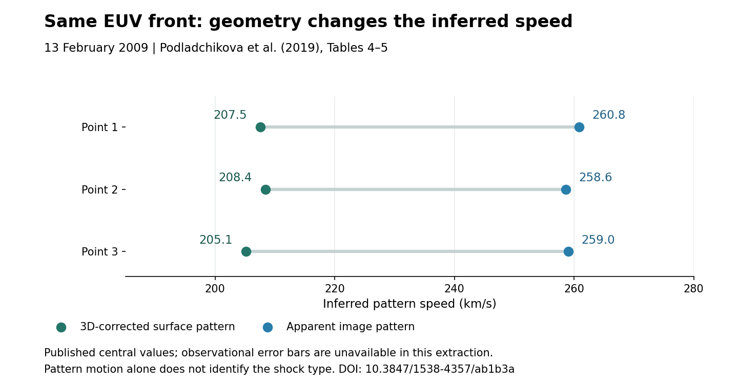
Save vector plot · SVG · Save plotted values and source · JSON
Click a Save link to choose the file name and folder when your browser supports it. Otherwise, Chrome uses its download settings. Press Ctrl+J to open Downloads, then choose Show in folder beside an ordinary download.
Filenames: RMO_EUV_2009_geometry.svg (figure) and RMO_EUV_2009_geometry.json (plotted values and source).
If you cannot find the downloaded file, the same values and source are also shown here.
{
  "event": "2009-02-13",
  "source": "T. Podladchikova et al. (2019), ApJ 877, 68",
  "doi": "10.3847/1538-4357/ab1b3a",
  "same_selected_patch_confirmed_by_author": true,
  "rows": [
    {
      "point": 1,
      "apparent_speed_km_s": 260.8333333333333,
      "surface_pattern_speed_km_s": 207.51,
      "reduction_relative_to_apparent_percent": 20.443450479233228
    },
    {
      "point": 2,
      "apparent_speed_km_s": 258.62333333333333,
      "surface_pattern_speed_km_s": 208.38166666666666,
      "reduction_relative_to_apparent_percent": 19.42657919496823
    },
    {
      "point": 3,
      "apparent_speed_km_s": 259.045,
      "surface_pattern_speed_km_s": 205.12,
      "reduction_relative_to_apparent_percent": 20.816846493852424
    }
  ],
  "result_sentence": "Geometry changes the inferred surface pattern speed; these tables alone do not determine an MHD shock type.",
  "family": null,
  "missing": [
    "local front normal and its uncertainty",
    "normal front speed in the selected local frame",
    "co-spatial density and thermal pressure on both sides",
    "plasma velocities and vector magnetic fields on both sides",
    "joint observational uncertainty"
  ],
  "limits": "Pattern motion is not plasma normal velocity; height change is not an independently recovered shock-normal speed. No new raw observations or assumed plasma state."
}
Save vector plot · SVG · Save plotted values and source · JSON
For a folder choice on every ordinary download: Chrome Settings → Downloads → Ask where to save each file before downloading. The selected folder is shown in the save dialog; the page does not receive its full system path. See Chrome download help.
| Published point | Apparent pattern (km/s) | Corrected surface pattern (km/s) | Reduction |
|---|---|---|---|
| 1 | 260.8 | 207.5 | 20.4% |
| 2 | 258.6 | 208.4 | 19.4% |
| 3 | 259.0 | 205.1 | 20.8% |
Values are calculated from published distances and a 600 s interval, rounded here for display. The source table's rounding is not a measurement error estimate; joint observational uncertainties are not supplied by this extraction.
What next? To attempt a local shock classification, we need the local front normal and its uncertainty, the normal front speed, plasma velocities, magnetic fields, density and thermal pressure on both sides, with their errors. Pattern motion is not plasma normal velocity.
The plot reproduces the published geometry comparison. No missing plasma state or magnetic field has been filled with an assumed mean, and no new solar shock classification is claimed.
See the front, watch its motion, then check where the model inputs come from.
Follow the evidence for the outer EUV front on 13 June 2010. At each step, ask what is known, what is assumed and what the next observation must resolve.
What comes next? Prepare matched 171, 193, 211 and 335 Å light curves for our sector, with explicit coordinates, observing times, background and front/CME passage. This is the next observational task; these matched curves have not yet been measured.
E05 · 16 FEBRUARY 2011 · CONDITIONAL MODEL COMPARISON
Veronig et al. (2011) · Hinode/EIS and SDO/AIA
They reproduce the same selected Doppler response and effective downstream density, using different assumed front and field geometries. This is a positive result about allowed models. It does not establish two waves in the event or identify an observed slow shock.
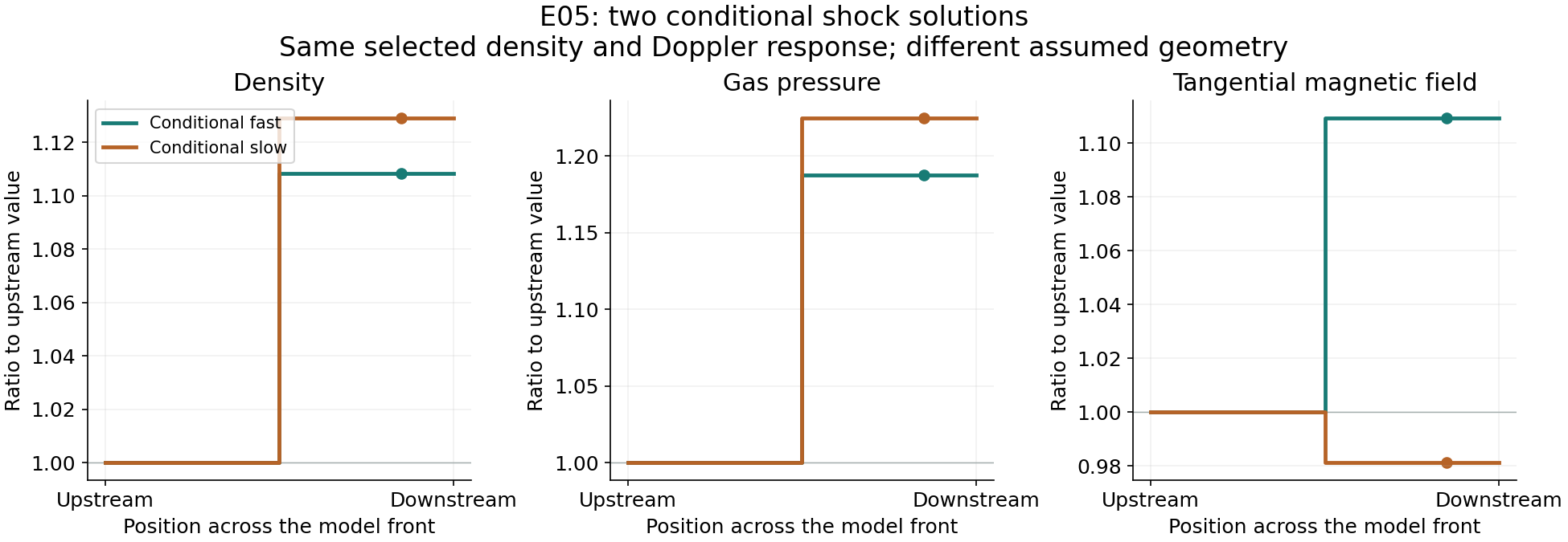
| Quantity | Fast model | Slow model | Origin |
|---|---|---|---|
| Normal front speed | 262.34 km/s | 185.5 km/s | ASSUMED / SOLVED in the model |
| Density ratio | 1.1084 | 1.1291 | ASSUMED / SOLVED in the model |
| Upstream density | 2.1207e+08 cm⁻³ | 2.0818e+08 cm⁻³ | ASSUMED / SOLVED in the model |
| Upstream temperature | 1.4792e+06 K | 1.461e+06 K | ASSUMED / SOLVED in the model |
| Upstream field magnitude | 0.92522 G | 3.7331 G | ASSUMED / SOLVED in the model |
| Front tilt below the local surface | 45 degrees | 60 degrees | ASSUMED / SOLVED in the model |
| Field–normal angle | 80 degrees | 30 degrees | ASSUMED / SOLVED in the model |
| Downstream electron density | 2.3505 × 10⁸ cm⁻³ | 2.3505 × 10⁸ cm⁻³ | R130 conditional effective density; assigning it to the downstream parcel is ASSUMED |
| Downstream temperature | 1.5849 MK | 1.5849 MK | ASSUMED central R130 temperature |
| Relative LOS response | +16.5596 km/s | +16.5596 km/s | MEASURED relative centroid; interpreting it as the parcel velocity jump is ASSUMED |
| Surface speed proxy | 371 km/s | 371 km/s | SOURCE-DERIVED EIS mean; associating it with exposure 25 is ASSUMED |
The saved EIS exposure is 14:28:40.646–14:29:25.646 UTC. R127–R130 retain the actual spectra, reference exposures, candidate registrations and density-response assumptions. The model additionally assumes that one parcel dominates the emission and that the local reference represents its upstream state.
The published 371 km/s value is a mean surface-track speed. It is not an independently measured instantaneous normal speed at this exposure.
A northward tangent is defined on the zero-height solar sphere at the selected patch. The fast model tilts the normal downward by 45°; the slow model uses 60°. For a planar front intersecting that surface, D = Vsurface (n · tangent). The normal points partly away from the observer, so a positive downstream normal response can produce the measured redshift.
Upstream plasma is stationary in both scenarios. The tangential magnetic direction is chosen along n × LOS; its associated velocity change does not contribute to the LOS signal. This is a strong geometry assumption, not a recovered coronal vector.
| Input | Origin | Meaning |
|---|---|---|
| Relative Fe XIII LOS centroid response | MEASURED | R127 relative emission-weighted centroid; not an upstream/downstream velocity jump. |
| Effective downstream electron density | SOURCE-DERIVED / RMO reduction | R130 conditional aperture density. Assigning it to the downstream parcel is assumed. |
| Surface speed proxy | SOURCE-DERIVED | Published EIS mean, not an instantaneous exposure25 normal speed. Treat as a scenario proxy;336 is the alternative AIA mean. |
| Normal | ASSUMED | Zero-height local sphere; northward tangent;45 degree downward tilt. Plane/surface intersection speed obeys D=Vsurface(n dot tangent). |
| Emission and reference | ASSUMED | One parcel dominates line emission; local reference is upstream; measured relative redshift equals the state-pair LOS jump. |
| Upstream flow and closure | ASSUMED | Upstream plasma stationary; pure fully ionized hydrogen; Te=Tp; isotropic ideal MHD;gamma=5/3; no extra heat flux. |
| Magnetic field | ASSUMED / SOLVED | Angle80 degrees to normal; tangential field along n cross LOS. Field magnitude and upstream pressure solved from conservation; neither is measured. |
| Downstream temperature | ASSUMED | Same central temperature scenario as R130 density inversion. |
The provenance table describes the reference fast model. In the slow comparison only the displayed geometry changes; field strength and upstream thermodynamics are solved again. The density uncertainty from R130 was not propagated into these exact state pairs.
Mass, three momentum components, two tangential induction conditions, normal-field continuity and energy conservation are checked. Both models have positive pressure and increasing entropy. The fast model crosses characteristic regions 1→2; the slow model crosses 3→4. No family label is passed to the diagnostic.
A second dimensional implementation checks the fluxes in SI units: the largest scaled residual is below 2 × 10⁻¹⁵ for these two models. The exact-synthetic input flag belongs only to the constructed model states. It is never attached to the observational records.
Pure ionized hydrogen, equal electron/proton temperatures, isotropic pressure and gamma = 5/3 are assumed. Conduction, unresolved emission and kinetic corrections are outside this closure.
The existence of both solutions survives an independent conservation check. Their preference is not established. A finite set of 72 geometry/speed/temperature scenarios is retained, including unclassified solutions; their counts are not probabilities or confidence intervals.
Most useful next constraint: an independent local front normal, together with the field direction/magnitude, would test the difference between these models. We have not calculated a justified angular-error threshold or proved that one measurement alone guarantees uniqueness.
A slower image speed is not itself a slow shock. Conversely, exceeding the sound speed does not by itself exclude a finite slow shock: its normal characteristic conditions must be checked.
Measured: spectra and a relative LOS response. Derived: an effective density with explicit atomic assumptions. Assumed: parcel association, front geometry, upstream rest and field orientation. RMO says: both a fast and a slow conditional shock exist. Still ambiguous: the actual local mode and whether a finite shock, smooth wave or more complex structure best describes the event.
The source study’s fast-mode interpretation remains credited. This model comparison is not a claim that the source interpretation is wrong. Code, data and scaling checks are included.
SW-C01 · SOLAR ORBITER · 30 AUGUST 2021
Suen et al. (2023), Event 3, CS2
The published slope is −0.697. The sign and strong field–flow trend agree qualitatively. This is an independently calculated comparison, not exact reproduction of the authors’ calibration or a new discovery.
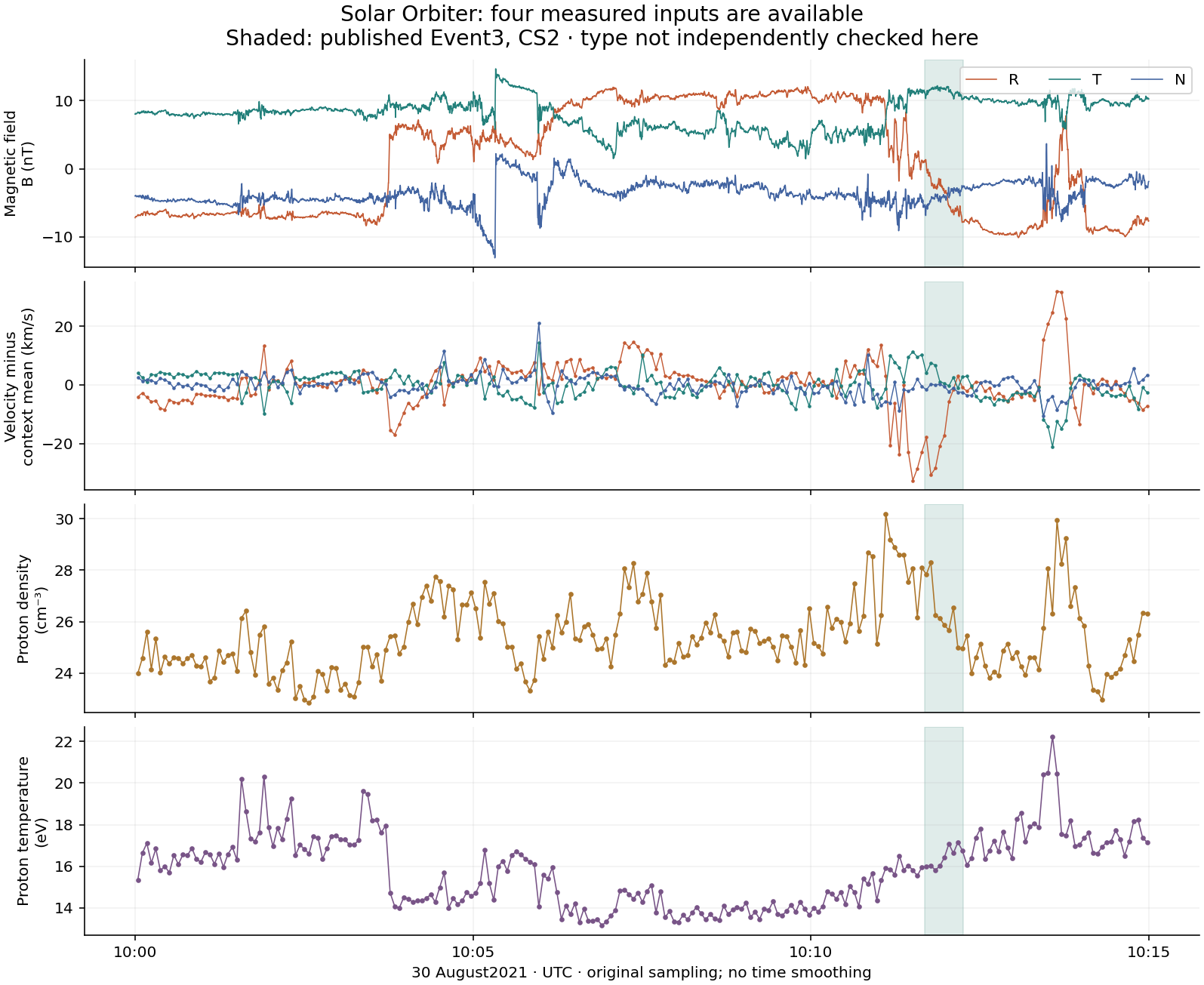
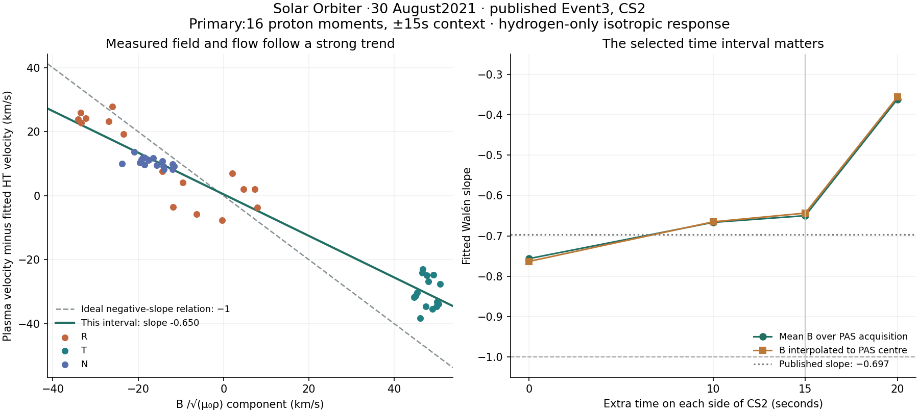
In a simple rotational discontinuity, the field turns and the plasma velocity changes on the Alfvén-speed scale: v − vHT = ± B / √(μ₀ρ). A slope near ±1 is one useful check. It does not replace the density, pressure, normal and conservation checks.
| Extra time on each side | MAG alignment | Proton samples | Slope | Component correlation |
|---|---|---|---|---|
| 0 s | acquisition mean | 9 | -0.756 | -0.982 |
| 0 s | center interpolation | 9 | -0.763 | -0.982 |
| 10 s | acquisition mean | 13 | -0.666 | -0.979 |
| 10 s | center interpolation | 13 | -0.665 | -0.979 |
| 15 s | acquisition mean | 16 | -0.650 | -0.975 |
| 15 s | center interpolation | 16 | -0.644 | -0.974 |
| 20 s | acquisition mean | 19 | -0.362 | -0.858 |
| 20 s | center interpolation | 19 | -0.356 | -0.853 |
These windows and the three components are dependent. The comparison range is not 1σ, a confidence interval or a calibrated observational error bound.
MAG V03 provides the measured field. SWA-PAS V03 provides proton density, velocity and temperature. MAG samples are averaged over each recorded 1 s PAS acquisition, at roughly 4 s cadence. The core has 9 proton moments; the primary extended interval has 16. Interpolation to the central time is retained as a comparison.
Hydrogen-only mass density and an isotropic Walén relation are assumed. Proton temperature does not supply the full electron/ion pressure. Composition, anisotropy and instrumental covariance are not fully known here. Exact CDF identities, quality flags and source-use metadata remain in the saved R130 input view and files.
Yes, for an explicitly constructed RD idealization anchored to the observed field rotation. Both Walén signs pass the exact local conservation and RD conditions. This checks the model against the solver without calling noisy data exact.
The idealization makes density, scalar pressure and field magnitude constant, retains the observed mean field directions, and chooses a normal with equal Bn. It also replaces the velocity jump by the ideal Alfvénic jump. For the negative sign, the required RMS vector correction to the two measured mean velocities is 10.18 km/s; for the positive sign it is 32.06 km/s. These corrections are not known measurement errors. A passing idealization is not a statistical fit to all observations.
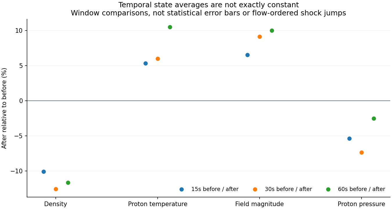
The primary minimum-variance normal has an intermediate/minimum eigenvalue ratio of only 1.26, so it is poorly constrained. The before/after field directions differ by about 40° with 15 s windows; density changes by about −10%, field magnitude by +6.5% and proton pressure by −5.4%. These are temporal contrasts, not measured shock-frame jumps with complete errors.
The fitted HT electric residual is 1.4% relative to the full convective field, but 50.7% relative to the demeaned-flow field. The small first number alone would overstate the quality of the frame. We retain both.
Result: Alfvénic / RD-compatible behaviour is supported. A unique exact ideal-MHD RD is not independently established. A reliable local normal, full pressure/composition and a defensible state/error model are the next useful inputs.
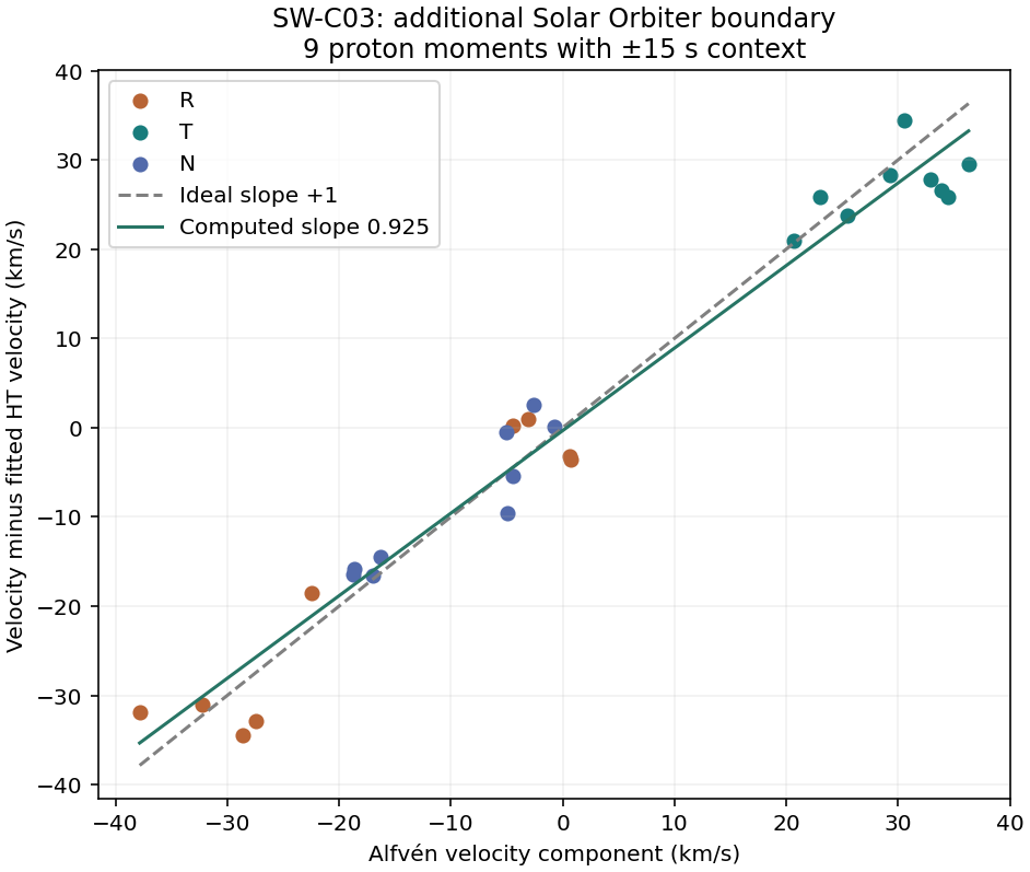
The independent calculation gives slope +0.925 in the reference interval, compared with the published +0.973. Extensions of 10 and 20 s give +0.776 and +0.974. We retain the reference interval and both alternatives; the closest coefficient is not selected after looking at the result.
This is a second direct field–flow check from the already saved CDFs. It supports Alfvénic behaviour, but its under-resolved core and uncertain normal prevent a unique exact-RD identification.
Suen et al. (2023); ESA Solar Orbiter Archive. MAG: Imperial College London and instrument team; SWA-PAS: MSSL-UCL/IRAP and instrument team. MAG V03 was generated after the source study; exact processing-version equivalence is not established.
Independent HT least squares, a Galilean-frame check, acquisition matching, a dimensional flux check of constructed states and all interval comparisons are saved. The observed data were not sent to an exact-only diagnostic as synthetic measurements.
Code, data and scaling checks are included.
RMO · ALL OBSERVATIONS AND A FINITE SOLAR-WIND COMPARISON
E05 now has two checked conditional shock solutions. SW-C01 has an independently calculated Alfvénic field–flow relation and an exact RD model comparison. One additional wind row, SW-C03, also has a direct CDF Walén check (+0.925). The other nine use published parameters; this is not ten new raw-data inversions.
| Record | Date | Result | What limits the interpretation | Source |
|---|---|---|---|---|
| E01 | 2007-05-19 | Speed definition checked The four channel peak speeds are not coeval states. The475 km/s track exceeds a262 km/s linear slow-wave phase-speed ceiling only if it is a plasma-frame normal speed and T≤2.5 MK; this does not exclude a finite slow shock. | Cadence and feature identity first; no four-mode comparison from four channels. | Long: thesis Chapter 4, Table 4.1; Long et al. 2008, doi:10.1086/589742 |
| E02 | 2010-07-27 | Two structures retained A slower image feature does not imply the slow MHD family. The source leading/trailing interpretations remain distinct. | Best remote candidate for testing a different trailing mode, but it needs a plasma-flow/field constraint. | Chen & Wu 2011, abstract; doi:10.1088/2041-8205/732/2/L20 |
| E03 | 2010-09-08/09 | Published fast-wave interpretation retained Wave-train tracks and the CME flank must remain separate. No numeric local MHD state is supplied by the current extraction. | A selected wave-train cut with local thermodynamics and field would support an informative next inversion. | Liu et al. 2012, Table 1 and Figures 1, 3–5; doi:10.1088/0004-637X/753/1/52 |
| E04 | 2011-02-15 | Thermodynamic consistency found Density increase6–9% predicts3.96–5.91% adiabatic heating for gamma5/3, overlapping the reported5–6%. This is compatible compression, not a unique fast/slow distinction. | EM, temperature, depth and filling-factor dependencies remain; no independent rectangular error box. | Vanninathan et al. 2015, methods/results; doi:10.1088/0004-637X/812/2/173 |
| E05 | 2011-02-16 | Fast and slow conditional solutions calculated Two constructed state pairs match the same chosen density, temperature and LOS response. Both pass conservation and their respective characteristic checks. Fast: X=1.108,Bup=0.925 G. Slow: X=1.129,Bup=3.733 G. | Normal tilt, source-speed association, upstream rest, emission parcel and field geometry are assumed. | Veronig et al. 2011, observations, diagnostics and Figures 1–5; doi:10.1088/2041-8205/743/1/L10 |
| E06 | 2011-06-07 | High-speed candidate retained Published mean800 km/s exceeds the262 km/s linear slow-wave ceiling under the speed/temperature assumptions. A slow shock has a different characteristic condition. Source model geometry and field are potentially useful. | Extract one actual model front point; do not substitute a global mean for its normal speed. | Kozarev et al. 2017, Section 3.1 and Figure 4; doi:10.1051/swsc/2017028 |
| E07 | 2013-12-12 | Linear phase-speed comparison only At a true normal speed450 km/s with stationary upstream plasma and T≤2.5 MK, a linear slow-mode phase speed is too small. A finite slow shock is not excluded by this sound-speed bound. These assumptions are not yet measured here. | This necessary speed check does not establish a fast shock or exclude an Alfvénic/image alternative. | Kozarev et al. 2017, Section 3.2; doi:10.1051/swsc/2017028 |
| E08 | 1998-06-13 | Accepted control complete The outer front and filament are different objects. A spectral non-detection cannot classify the front. | Keep the accepted association control; no forced model completion. | Madjarska et al. 2015; Harra & Sterling 2003; accepted project audit; doi:10.1051/0004-6361/201424754 |
| E09 | 2015-06-22 | Published slow-shock model benchmark The source conductive model supplies a positive slow-shock comparison associated with IRIS observations. It has not been independently reproduced with the adiabatic RMO closure. | Reproduce the energy flux including conduction before importing the model as a tested RMO state pair. | Ye et al. 2026, Figures 4–6 and thermal-conduction discussion; doi:10.1038/s41467-026-75039-z |
| E10 | 2011-01-27 08:45 UT | Linear phase-speed comparison only The341 km/s mean exceeds the linear slow-wave ceiling262 km/s under the same normal-speed, zero-flow and temperature assumptions. Finite slow shocks remain a separate check. The610 km/s initial fit is a different quantity. | Choose one epoch and model geometry; no mode from flare class. | Muhr et al. 2014, Table 4; doi:10.1007/s11207-014-0594-7 |
| E11 | 2010-06-13 | Conditional slow solution already checked The saved F1 completion admits a slow shock for the inner feature. It is a positive model-existence result; its unknown intermediate flow/state are not measurements. | Outer radio constraints are not transferred to the inner front. Actual fast, Alfvénic and material alternatives remain open. | Project R119–R122 saved reports and their source receipts are controlling; Ma et al. 2011 is one input source. |
| G2009 | 2009-02-13 | Geometry result reproduced The matched published surface speed changes from about260 to207 km/s after correction. | Positive geometry result; local field and plasma state are still needed to identify a family. | T. Podladchikova et al. 2019, Tables 4–5; doi:10.3847/1538-4357/ab1b3a |
The speed-only rows compare an explicit linear slow-wave ceiling, about 262 km/s for the stated hydrogen/temperature scenario. This is not a universal coronal bound and does not exclude a finite slow shock. No row is promoted to fast just because another family was not demonstrated.
| Case / spacecraft | Time (UTC) | Published inputs used | Screening result | Source |
|---|---|---|---|---|
| SW-C02 · Solar Orbiter | 2021-08-10 07:45:50–07:48:45 | {"published_Walen_slopes": [-0.254, -0.497, 0.309]} | None of the three published slopes reaches magnitude0.5. Retain as a contrast case, not a pure-RD confirmation. The source discusses reconnection; a slope cutoff alone is not a mode test. | Event1, Figures1–2 |
| SW-C03 · Solar Orbiter | 2021-08-30 10:21:24–10:21:28 | {"published_Walen_slope": 0.973, "computed_Walen_slope": 0.924808549994076, "extended_proton_samples": 9, "core_proton_samples": 1} | Independent same-day CDF check gives slope+0.925 with15s context. A strong positive Alfvénic relation is reproduced; the boundary core itself has only one proton sample. 10/15/20s extensions give slopes+0.776/+0.925/+0.974. These are interval choices, not errors. A full local discontinuity classification remains conditional. | Event2, Figures3–4 |
| SW-C04 · PSP | 2018-10-27 04:42:00 | {"duration_s": 51.9, "magnetic_shear_deg": 133, "across_exhaust_velocity_to_Alfven_shear_ratio": 0.1} | Published reconnection exhaust; an individual boundary must be selected before testing RD or slow-shock conditions. The quoted shear ratio across the exhaust is not the boundary Walén regression slope. No slow-shock label inferred. | Table1, events1,2,7 respectively |
| SW-C05 · PSP | 2018-10-29 19:07:30 | {"duration_s": 38.4, "magnetic_shear_deg": 120, "across_exhaust_velocity_to_Alfven_shear_ratio": 0.3} | Published reconnection exhaust; an individual boundary must be selected before testing RD or slow-shock conditions. The quoted shear ratio across the exhaust is not the boundary Walén regression slope. No slow-shock label inferred. | Table1, events1,2,7 respectively |
| SW-C06 · PSP | 2018-10-31 12:14:30 | {"duration_s": 32.4, "magnetic_shear_deg": 97, "across_exhaust_velocity_to_Alfven_shear_ratio": 0.56} | Published reconnection exhaust; an individual boundary must be selected before testing RD or slow-shock conditions. The quoted shear ratio across the exhaust is not the boundary Walén regression slope. No slow-shock label inferred. | Table1, events1,2,7 respectively |
| SW-C07 · Solar Orbiter | 2021-06-13 10:08:38 | {"catalogue_id": "SHK-2021061310", "mms": 1.3, "ma": 1.45, "rB": 1.5, "rGas": 1.7, "n_u": 5.9, "theta_Bn": 82.0, "necessary_fast_screen_pass": true} | Published fast-shock candidate passes the tabulated upstream super-fast/compressive screen. Rounded, model-derived catalogue means. Downstream characteristics and all jump residuals are not supplied by this row. Subcritical shock | SHK-2021061310 |
| SW-C08 · Solar Orbiter | 2021-07-18 17:57:50 | {"catalogue_id": "SHK-2021071817", "mms": 1.9, "ma": 2.6, "rB": 2.0, "rGas": 2.0, "n_u": 23.5, "theta_Bn": 78.0, "necessary_fast_screen_pass": true} | Published fast-shock candidate passes the tabulated upstream super-fast/compressive screen. Rounded, model-derived catalogue means. Downstream characteristics and all jump residuals are not supplied by this row. Strong overshoot | SHK-2021071817 |
| SW-C09 · Solar Orbiter | 2021-07-19 08:28:02 | {"catalogue_id": "SHK-2021071908", "mms": 1.9, "ma": 2.4, "rB": 1.5, "rGas": 1.7, "n_u": 20.0, "theta_Bn": 70.0, "necessary_fast_screen_pass": true} | Published fast-shock candidate passes the tabulated upstream super-fast/compressive screen. Rounded, model-derived catalogue means. Downstream characteristics and all jump residuals are not supplied by this row. High frequency activity near ramp | SHK-2021071908 |
| SW-C10 · ACE / Cluster / Wind | 2002-02-02 | {"spacecraft_count": 3} | The authors reconstruct mixed slow/intermediate behaviour. It is a useful compound-boundary comparison, not a pure standard-jump control. One physical event, not three independent discoveries; the source explicitly discusses imperfect standard jump conditions. | Teh et al.2009, Figures2–4, section4 |
| SW-C11 · PSP | 2024-09-30 11:52–12:39 | {"repeated_crossings": 12} | High-priority slow-shock reference, with an Alfvén-speed definition check required before importing its table. Repeated crossings of one exhaust; anisotropic thermodynamics. Source identification is retained, not claimed as an independent RMO result. | Sun et al.2026 preprint, Table1 and AppendixC |
Repeated boundaries within one exhaust, multiple instruments and multiple spacecraft are not counted as independent discoveries. Selection covers contrasting diagnostics; it is not a blind survey or an estimate of occurrence rates.
Sun et al. (2026), preprint report slow/rotational compound boundaries on 30 September 2024. Their tabulated slow Mach numbers straddle unity. Before using those numbers in RMO, the Alfvén-speed convention and anisotropic closure need to be aligned.
| Crossing | Mslow upstream / downstream | MA upstream | θ upstream | MA,n if MA uses |B| |
|---|---|---|---|---|
| LO | 1.09 / 0.67 | 0.57 | 85.7° | 7.60 |
| LI1 | 1.39 / 0.96 | 0.97 | 85.1° | 11.36 |
| LI2 | 1.08 / 0.79 | 0.80 | 88.1° | 24.13 |
| LI3 | 1.21 / 0.88 | 0.89 | 88.4° | 31.87 |
| LI4 | 1.35 / 0.73 | 0.97 | 88.9° | 50.53 |
| LI5 | 1.35 / 0.80 | 0.98 | 86.1° | 14.41 |
| TI1 | 1.80 / 0.57 | 0.97 | 89.0° | 55.58 |
| TI2 | 1.52 / 0.60 | 0.73 | 79.6° | 4.04 |
| TI3 | 1.42 / 0.78 | 0.89 | 76.6° | 3.84 |
| TI4 | 1.39 / 0.99 | 0.81 | 72.0° | 2.62 |
| TI5 | 1.34 / 0.83 | 0.78 | 60.7° | 1.59 |
| TO | 1.23 / 0.86 | 0.52 | 88.3° | 17.53 |
AppendixC prints vA=|B|/sqrt(mu0 rho), while the ideal-MHD slow branch needs vA,n=|Bn|/sqrt(mu0 rho). Taken literally with the listed angles, the supplied Mach numbers do not share the expected cslow≤vA,n ordering. If the table MA is already normal, the simple crossing inequalities pass. Clarify the definition and anisotropic closure before reuse. This is not a claim that the observed boundaries cannot be slow shocks.
This calculation identifies a definition issue to resolve, not a new physical identification or a rejection of the authors’ interpretation. Original source tables and the arithmetic are saved.
Reproduced: our calculation independently recovers a stated measurement or physical relation. Conditional: a complete specified model satisfies the data constraints we actually used. New observational identification: data establish a type not previously established for that same feature, after competing admissible explanations and uncertainty are addressed.
This stage supplies positive reproduced and conditional results. It does not claim a new observed slow shock, an unknown fast shock, or a newly discovered rotational discontinuity.
For E05, the field/normal difference between two explicit models is now concrete. For new in-situ work, a boundary with adequate plasma cadence and an unambiguous pressure/normal convention is more useful than an impressive image alone.
The frozen SERPENTINE file used here contains 61 rows, of which 51 have the selected screen inputs. Only the first three complete chronological rows enter the ten-case selection. This snapshot is not the later 100-shock survey or the current live catalogue. Frozen catalogue and credit. All prior visual viewers and event cards remain available in QuickLook.
Code, data and scaling checks are included.
E05 · 16 FEBRUARY2011 · STEP3: COLLECT PLASMA CONSTRAINTS
Veronig et al. (2011) · Hinode/EIS and SDO/AIA
The formal interval is about −8% / +8%. It includes spectral noise with the model fixed. Calibration, atomic data, radiation and unresolved plasma structure are not included in that interval.
This is an effective aperture density. Shock compression remains unknown.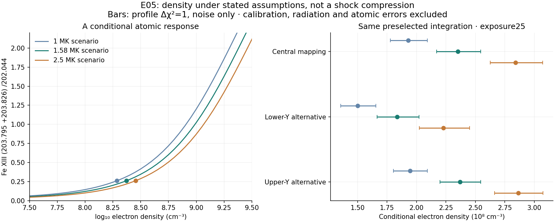
At the central mapping, changing only the assumed temperature from1.0 to2.5 MK gives about1.93–2.84 ×10⁸ cm⁻³. The full set of plotted mapping/temperature combinations gives about1.50–2.86 ×10⁸ cm⁻³. These are scenario values, not measured lower and upper limits.
| Quantity | Value / result | Origin | Uncertainty and limits |
|---|---|---|---|
| Electron density | 2.35 ×10⁸ cm⁻³; about −7.7% / +8.2% | DERIVED HERE, CONDITIONAL | Profile Δχ²=1, noise only; all model assumptions fixed. Not a complete1σ error budget. |
| Temperature | 1.585 MK central; 1.0 and2.5 MK comparisons | ASSUMED scenarios | These temperatures are not measured bounds for the selected front. |
| Atomic model | CHIANTI11.0.2 subset; ChiantiPy0.16.0 | SOURCE MODEL | 749 levels, electron/proton excitation and radiative decay. File versions and hashes are retained. |
| Radiation and plasma mixture | No incident photospheric radiation; one effective density/temperature | ASSUMED | Photoexcitation and unresolved emitting components can change the inferred density. |
| Relative response calibration | Stored EIS pre-flight radiometric conversion | SOURCE-DERIVED instrument calibration | Calibration evolution and its uncertainty have not been included. |
| Compression ρ₂/ρ₁ | Unknown | UNKNOWN | No identified upstream/downstream density pair; the aperture may mix front and background. |
| Local MHD type | No new independent identification | UNRESOLVED | Normal geometry, absolute normal flow, magnetic constraints and a state pair remain incomplete. |
The two Fe XIII components near203.8Å do not have a fixed intensity ratio at every density. We now fit their ratio together with density, using the atomic response. At the central solution the component ratio is about0.453. The earlier fixed0.40 fit remains saved as R129.
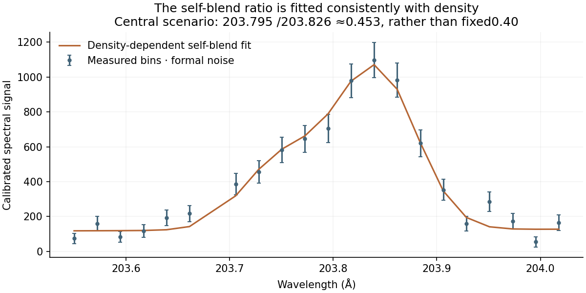
The model uses the Fe XIII transitions1→20,3→24 and3→25:202.044,203.795 and203.826Å in the downloaded atomic files. The fitted wavelength offsets are free within the retained bounds. Energy radiances are compared, using the same line-area convention as the saved EIS fits.
The joint fit uses the202Å line area with its formal variance and the native203Å spectral bins. At each trial density, the line amplitudes, width, centroid and background are adjusted. Profile limits use Δχ²=1; the Gaussian approximation for the202Å area is retained. The three temperature scenarios and three existing mappings all pass the retained fit-quality limits.
Direct atomic calculations at the fitted central densities agree with the tabulated interpolation to better than0.002% in line ratio. All level populations are nonnegative and normalized. This checks implementation consistency; it does not bound atomic-rate or calibration error.
The response assumes an optically thin Maxwellian plasma, electron and proton excitation, spontaneous radiative decay and no external radiation. Inter-ion population correction and continuum emission are not used. The proton/electron ratio follows the saved CHIANTI ionization and abundance tables. Source code and assumptions are recorded.
R129 did not establish a secure positive line-ratio change across the retained mappings. R130 does not turn that result into a detected density increase. Neither stage provides an upstream/downstream compression. The source study’s fast-mode interpretation remains credited separately from this local reconstruction.
eis_20110216_140955, saved from R126. No new EIS reduction is claimed.Code, data and scaling checks are included.
SOLAR WIND · SEPARATE METHOD COMPARISON
Suen, Owen, Verscharen, Horbury, Louarn & De Marco (2023)
This stage checks data availability. RMO has not yet independently reproduced the discontinuity classification.
The authors identify an Alfvénic rotational discontinuity at Event3, CS2, on30 August2021,10:11:41–10:12:15 UTC. Their Walén slope is−0.697. We select this34s boundary because it has more proton samples than the5s CS1 boundary. Their interpretation and our checks remain separate.
| Input | Units | Samples | Cadence | Origin | Error information |
|---|---|---|---|---|---|
| B_RTN | nT | 7200 in15min; 272 withinCS2 | 0.125s | MEASURED / team-derived moments | No per-sample error array for this quantity in these files |
| N | particles cm^-3 | 225 in15min; 9 withinCS2 | 4s | MEASURED / team-derived moments | No per-sample error array for this quantity in these files |
| V_RTN | km/s | 225 in15min; 9 withinCS2 | 4s | MEASURED / team-derived moments | No per-sample error array for this quantity in these files |
| T | eV | 225 in15min; 9 withinCS2 | 4s | MEASURED / team-derived moments | No per-sample error array for this quantity in these files |
The PAS integration spans about1s at a4s cadence. The pressure tensor, temperature components and spacecraft velocity are also retained. These extra fields may help check anisotropy and reference frames; they have not yet been used to close a transition model.
A classical ideal-MHD rotational discontinuity changes field and flow directions without a density or scalar-pressure jump. A slow shock is a different candidate. A Walén slope alone is not a complete conservation-law check.
ESA Solar Orbiter Archive: solo_L2_mag-rtn-normal_20210830_V03.cdf and solo_L2_swa-pas-grnd-mom_20210830_V03.cdf. MAG data: Imperial College London, T. Horbury and team; SWA-PAS: MSSL-UCL/IRAP, C. Owen and team. Exact files, metadata, source terms and checksums are saved.
The context contains no missing values in the four displayed streams. MAG has quality flag3 and detailed bitmasks128/140; the CDF documents removed interference and heater flags. Its metadata makes publication use subject to PI approval. SWA metadata requests consultation with MSSL-UCL. These conditions are retained; this preview does not claim publication clearance. Quality flags are not statistical errors.
MAG V03 was generated in2024, after the source study. We have not established that its processing matches the authors’ version.
Yes. ACE SWEPAM provides solar-wind plasma data at64s resolution, and ACE MAG provides magnetic-field products including1s and16s averages. A suitable event needs enough samples on both sides and a documented interpretation. No ACE event is downloaded or classified in this stage.
Separate method comparison; the12 core observational records remain unchanged. Code, data and scaling checks are included.
E05 · 16 FEBRUARY 2011 · DENSITY-SENSITIVE LINE RATIO
Veronig et al. (2011) · Hinode/EIS spectra · SDO/AIA image context
The line ratio can be measured. A density jump at the front is not established.
The central line-ratio change is +12% ±9 percentage points at the selected integration. The ± value is formal1σ, not a full error budget. Other retained aperture mappings give smaller or negative central changes. We keep compression unknown.
Step is the focus reached in saved work, not a count of fully known inputs. Literature review, direct reconstruction and completed controls remain distinguished.
| Card | Step | Current status |
|---|---|---|
| E01 | 1 · Match the observations | Published speed comparison retained. Match the feature, cadence and interval before comparing modes. |
| E02 | 1 · Match the observations | Two published image features kept separate. Local association and plasma constraints remain open. |
| E03 | 1 · Match the observations | Event identity resolved. Select one wave-train track and separate it from the CME flank. |
| E04 | 3 · Collect plasma constraints | Published density and temperature constraints reviewed. Their emission-model assumptions remain explicit. |
| E05 | 3 · Collect plasma constraints | Line ratio measured; compression still unknown. Geometry and normal flow remain conditional. |
| E06 | 2 · Check geometry and motion | Published front tracking and model geometry retained. A local state pair remains incomplete. |
| E07 | 2 · Check geometry and motion | Published front speed retained. Local plasma and thermodynamic inputs remain missing. |
| E08 | 1 · Match the observations | Association control complete and retained. The filament spectrum is not assigned to the outer front. |
| E09 | 3 · Collect plasma constraints | Published spectra and model interpretation reviewed. Energy-closure compatibility still needs checking. |
| E10 | 2 · Check geometry and motion | Published speed definitions retained. Local normal geometry and plasma-frame information remain open. |
| E11 | 5 · Check what holds | Bounded review complete. The inner feature remains unresolved; no unique mode is claimed. |
| G2009 | 2 · Check geometry and motion | Published geometry comparison reproduced. This is not a full MHD inversion. |
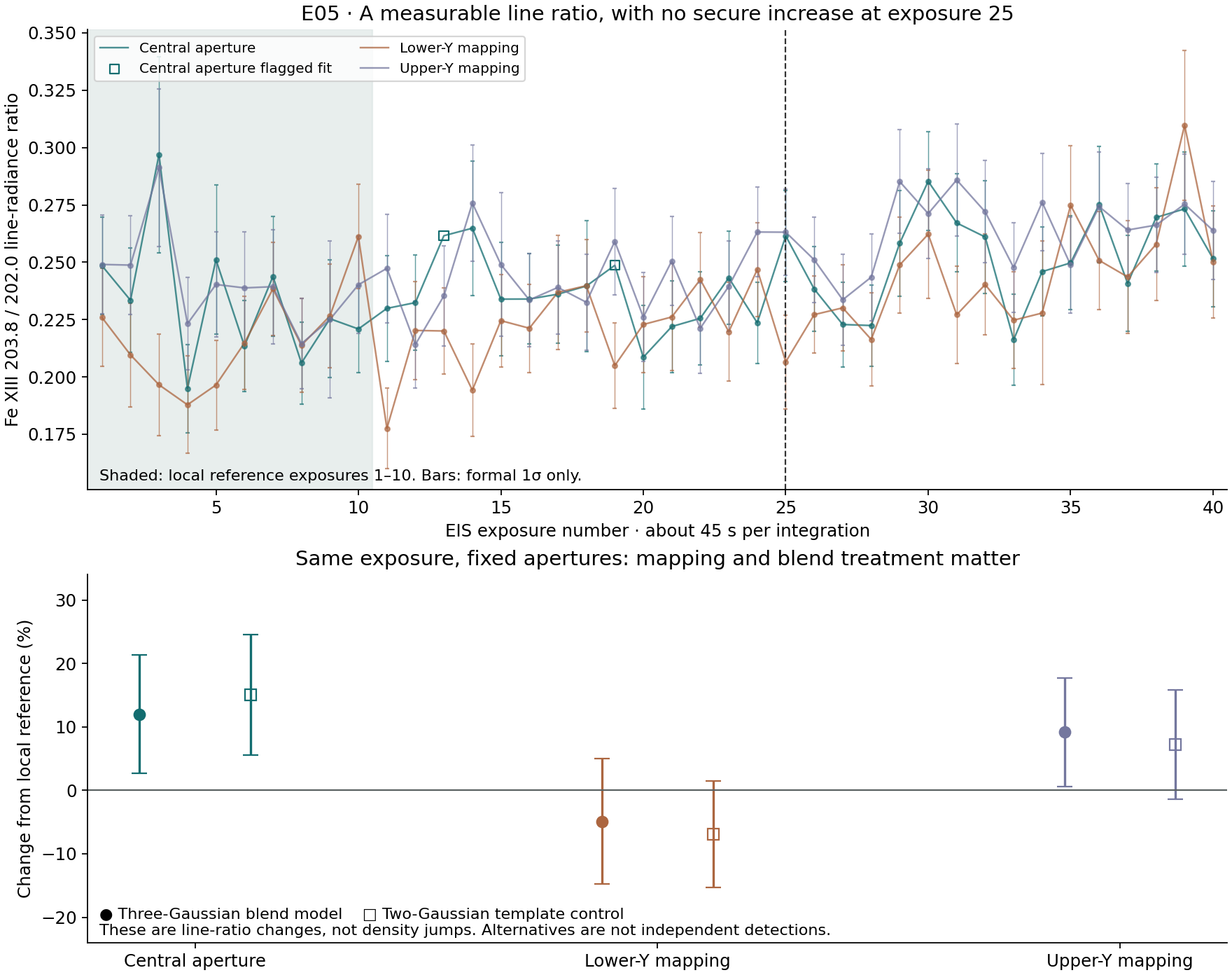
Read this carefully: “+12%” refers to a change of the line ratio. It is neither “density rose by12%” nor “compression X=1.12”. The response from line ratio to electron density is nonlinear and needs an atomic model. A density change in an emission-weighted aperture still needs an identified upstream/downstream pair before it can be used as X.
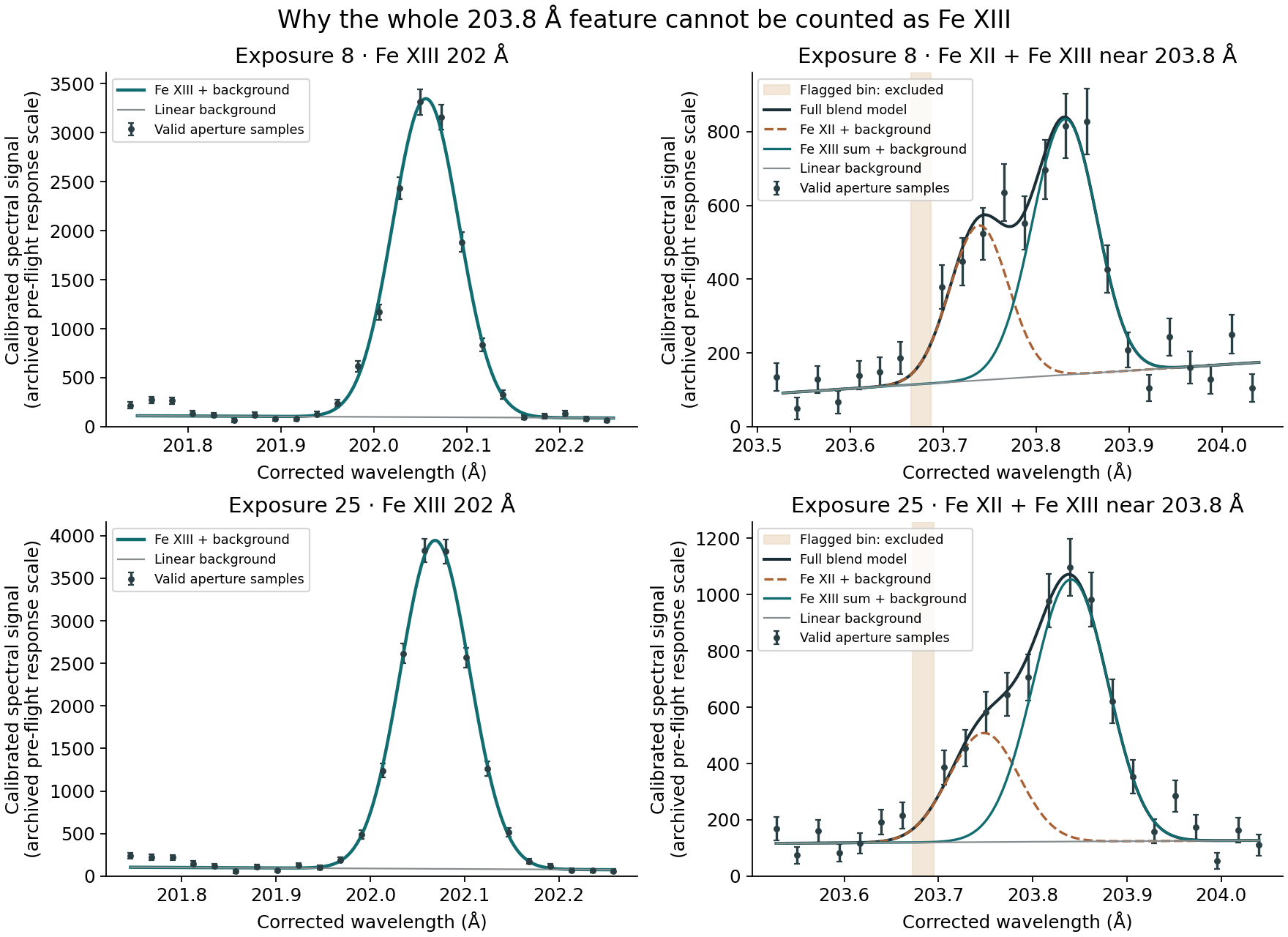
The primary model uses three common-width Gaussians: Fe XII203.728 and the Fe XIII203.797/203.828 pair, with fixed separations and a Fe XIII component ratio0.40; the background is linear. This follows the blend treatment in Young et al., section5.5. The component ratio is a line-model assumption, not an E05 density measurement.
A second fit uses the pinned NRL EISPAC two-Gaussian template form. The fitted Fe XIII area changes modestly. Neither treatment gives a secure increase in this selected comparison. These two models do not exhaust all possible blend systematics.
| Quantity | Value / result | Origin | Source / method | Uncertainty / assumption | Use in RMO |
|---|---|---|---|---|---|
| Selected area and time | E05 · 16 February 2011; central Fe XIII202 rows334–338; exposure25:14:28:40.646–14:29:25.646 UTC | MEASURED metadata + ANALYSIS CHOICE | R125–R127 native EIS timing, registration and fixed apertures | About45s integration; alternative mappings retained. The exact published extraction is not recovered. | Compare a named candidate region. Equal times alone do not establish the same emitting plasma. |
| Fe XIII203.8 /202.0 line ratio | 0.261 ±0.020 at exposure25; local reference0.233 ±0.008 | DERIVED HERE from measured EIS spectra | Stored pre-flight response; constrained three-Gaussian blend fit; five-row aperture | Formal1σ noise and local fit covariance only. The numerator excludes the fitted Fe XII contribution. | A spectral observable sensitive to density; it is not itself electron density. |
| Relative line-ratio response | +12.0% ±9.3 percentage points at exposure25 | DERIVED HERE | Ratio at25 divided by the ratio of mean line radiances in exposures1–10, minus1 | Formal1σ only. Shared reference covariance is included in the full time series; reference points are correlated. | A small positive central estimate, about1.3 formal standard errors from zero; no secure increase established. |
| Aperture mapping alternatives | Primary model: −4.9% ±9.9 points and +9.2% ±8.5 points | ANALYSIS CHOICES retained from R126 | Same fixed lower-Y and upper-Y alternatives; no peak selection | Formal1σ within each case. These overlapping alternatives are not independent measurements or a confidence interval. | The sign of the central estimate is not stable across the retained mappings. |
| Blend-model comparison | Central two-Gaussian control: +15.0% ±9.5 points | ASSUMED line shape + DERIVED HERE fit | Pinned NRL EISPAC template form: common width, separate centroids, constant background | A modelling comparison, not a second independent observation; it does not define full systematic error bounds. | The small increase remains inconclusive. |
| Spectral-window spatial offset | 203Å sampled0.141 detector pixel below202Å at the same sky Y | SOURCE-DERIVED instrumental correction | Stored HDF5 CCD offsets; fractional pixel-overlap weights | Piecewise uniform intensity within a detector pixel. Absolute EIS–AIA mapping is still provisional. | Use matched aperture areas; the central response changes by about1.1 percentage points versus unshifted rows. |
| Spectral aggregation | Same five-row area, 40 native integrations; no time smoothing | ANALYSIS CHOICE | Coadd calibrated spectral bins; retain native-row results and all masks | Maximum wavelength spread inside one combined bin0.000519Å, compared with0.0223Å sampling. Row noise treated as independent. | Improves weak-line precision without widening the selected region or pooling different event times. |
| Electron density | Not assigned in this stage | UNKNOWN numeric value | A versioned atomic ratio-to-density response has not been applied | Requires stated atomic data, temperature/radiation assumptions and relative response calibration; line-of-sight mixtures remain possible. | Do not insert a guessed density from the observed line-ratio value. |
| Compression X = ρ₂/ρ₁ | Not determined | UNKNOWN | No matched upstream/downstream density pair is established | Local temporal changes need not be a shock jump. Electron-density ratio equals mass-density ratio only with appropriate composition/ionization assumptions. | Keep X unassigned. This result does not show that compression is absent. |
| MHD type for this local reconstruction | No new independent identification | UNRESOLVED | R128 geometry/motion limits and this spectral-ratio result | Normal front speed, absolute normal flow, magnetic constraints and a state pair remain incomplete. | Credit the published fast-mode interpretation; do not select or exclude a family from this ratio alone. |
What would make compression usable? Identify the front and background contributions in the same sampling area and time interval, then apply a documented atomic ratio-to-density response with its assumptions. This separates a density diagnostic from a claim about an upstream/downstream jump. The earlier unknown normal geometry, background flow and magnetic constraints still matter.
Source context: Veronig et al. (2011) already discusses the difficulty of detecting a small density enhancement at the EUV front. This local reconstruction keeps that interpretation separate from its own fixed-aperture measurements.
eis_20110216_140955.head.h5 and eis_20110216_140955.data.h5, retained from R126. Native windows04 and05, source hashes and processing choices are included.Saved outputs include native-row and aperture fits, covariance matrices, masks, CCD weights, both line models, all40 exposures, the comparison table, source receipts and verification. Code, data and scaling checks are included.
Result: a qualified density-sensitive spectral observable. Compression and independent MHD identification remain open.
E05 · 16 FEBRUARY 2011 · IMAGE GEOMETRY AND PLASMA MOTION
Veronig et al. (2011) · Data and sources
The spectra measure a change along our line of sight. The images locate a candidate region, but they do not yet determine the plasma speed through the front.
+16.6 ± 1.1 km/s redward, relative to the earlier local Fe XIII signal. The error is formal 1σ only.
18.7 ± 1.3 km/s downward if the change is purely radial at the assumed surface location. This is a direction assumption, not a new measurement.
The 3D front normal, transverse velocity changes, background normal velocity and local normal front speed. A unique MHD family is not established here.
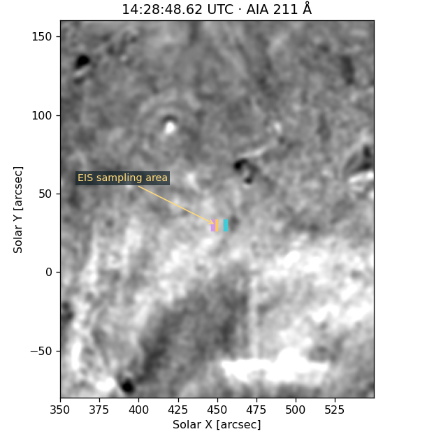
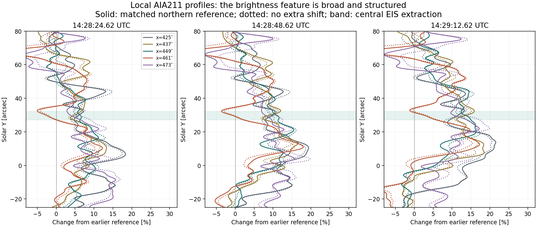
Change: northern reference match
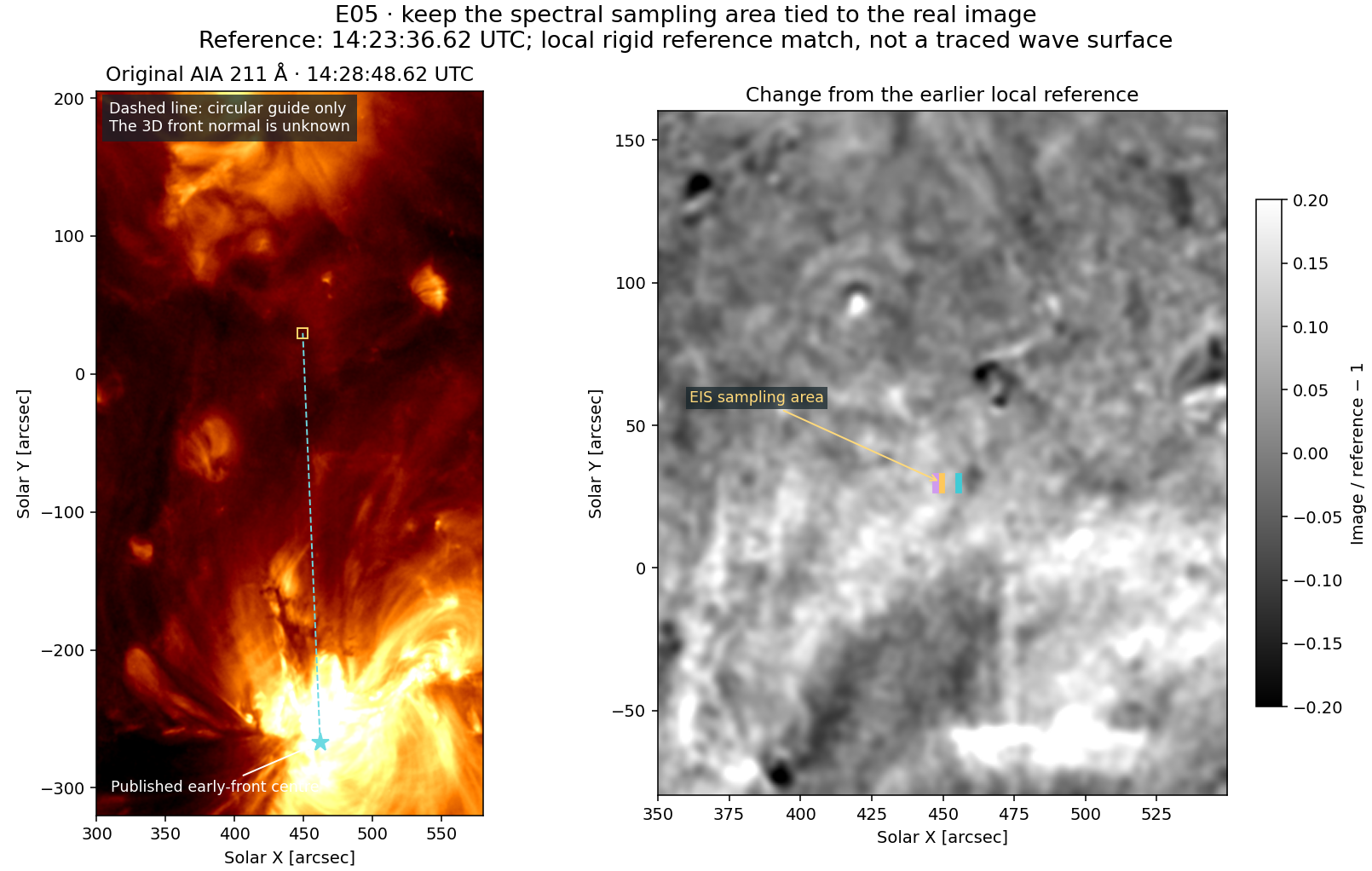
SDO/AIA 211 Å. Change views show image/reference − 1 on the same clipped scale, −0.20 to +0.20. Reference: 14:23:36.62 UTC. The markers are the three R127 sampling alternatives. No line drawn on these images is a fitted front. Playback is illustrative; images are 24 seconds apart.
The earlier frame makes a broad, structured brightness change easier to see near the candidate area. We have not obtained a unique local ridge or front normal from these three images. The image intensity and the Fe XIII centroid weight the emitting plasma differently.
We added exactly one native AIA 211 Å file, at 14:23:36.62 UTC, and used the three later files already saved at R125. Every frame is divided by its exposure time and mapped with the same saved master pointing and WCS method. We apply equal Gaussian smoothing, σ = 1.5 arcsec, to the reference and later images before forming the ratio. There is no temporal smoothing or conversion from brightness to density.
Small rigid reference offsets are fitted using northern structure at X = 350–550″, Y = 90–160″. The selected spectral pulse near Y = 30″ is excluded. Separate lower and upper northern regions and a no-extra-shift view are retained. Positive fitted offsets mean sampling the earlier reference at X + ΔX, Y + ΔY. They do not move the EIS aperture. This is a local matching aid, not certified solar derotation or absolute cross-instrument registration.
The combined northern offsets are about −0.7 to −0.9″ in X and +0.1″ in Y. A high correlation score does not give an uncertainty on the wavefront position. The exact offsets, windows and scores are saved.
Two of the later AIA integrations lie within the 45-second EIS exposure 25. The source study describes a typical intensity response one EIS step after the velocity pulse. We do not impose that lag on this selected aperture or interpret the short image sequence as a simultaneous plasma-state pair.
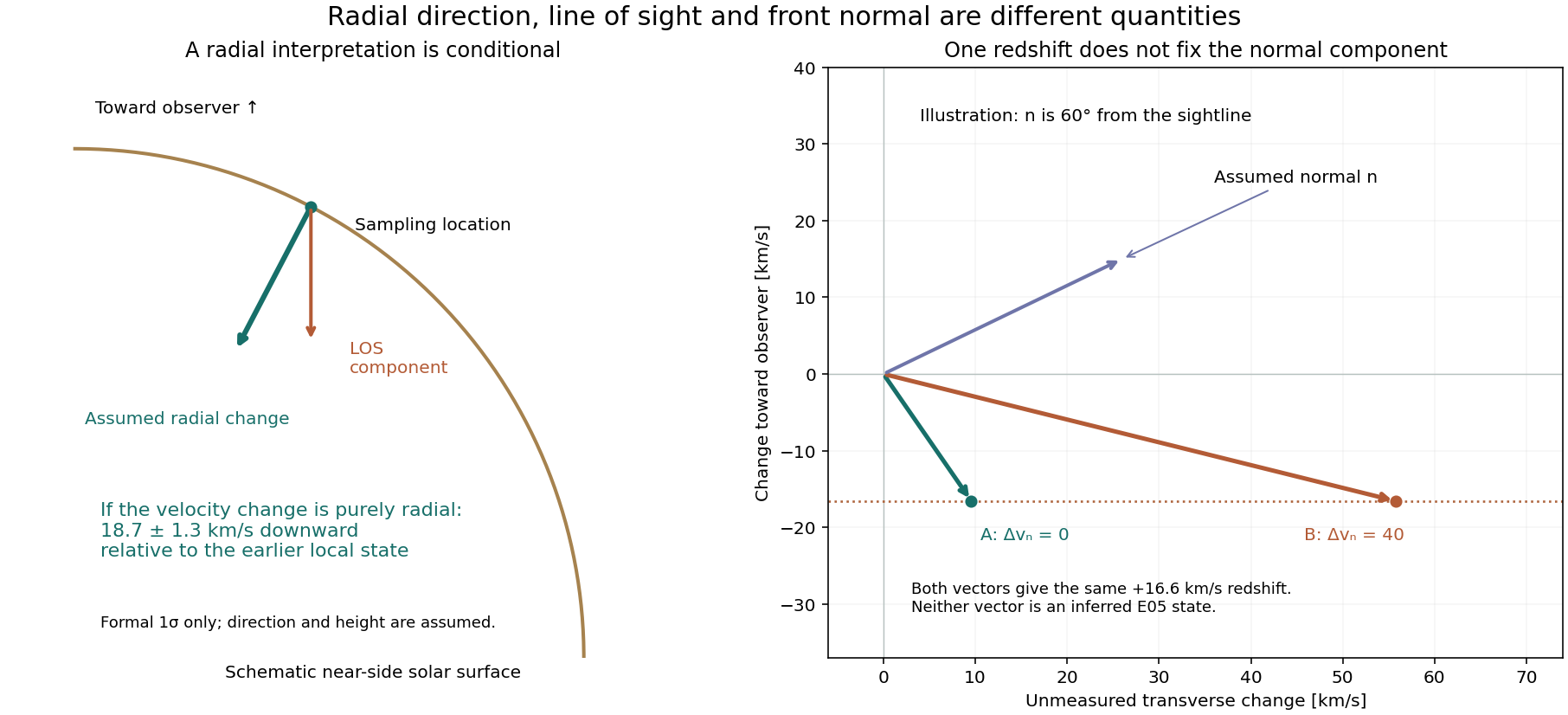
The location on the disk gives a radial projection of about 0.886 under the stated height assumption. Dividing the redshift by this factor gives the conditional downward change. It does not tell us that the plasma moves radially or that the solar radial direction is the wavefront normal.
Even with a known front normal, a single Doppler measurement generally leaves transverse motion unconstrained. To obtain the absolute normal flow, we would also need the normal velocity of the reference plasma. A more precise measurement of the same LOS shift alone cannot supply those missing components.
Let ell point toward the observer; positive d means redshift. For one identified emitting component, the relative response is
d = −ell · Δv + εrel.
Split the change into a component along the unit front normal n and a tangential component:
d = −μn Δvn − ell · Δvt + εrel, μn = ell · n.
The tangential term can contribute to the Doppler signal. Setting it to zero is an additional physical assumption. If n is exactly parallel to the sightline, the normal change can be read from d under the same emitting-component and calibration assumptions; the absolute background velocity is still needed. The example above keeps n fixed and gives two vectors with the same d but different Δvn; it is a demonstration of non-uniqueness, not a search for event solutions.
For the absolute velocity and our incoming front-frame convention:
vn(t) = vn,ref + Δvn; wi,n = Dn − vi,n.
The reference normal velocity, local normal front speed and matched upstream/downstream states remain unknown. We do not subtract the published image speed from the Doppler shift.
The radial illustration uses the near-side ray–sphere intersection, AIA observer distance and solar radius, and height = 0. The radial viewing angle is about 27.6°. It is not a field angle or an observed front-normal angle. The fitted centroid is emission-weighted: changes in the contributing structures can move it without tracking the velocity of one parcel.
| Quantity | Value / result | Origin | Source / method | Uncertainty meaning | What this allows |
|---|---|---|---|---|---|
| Relative Fe XIII shift | +16.6 ± 1.1 km/s, redward; exposure 25 | DERIVED HERE from measured spectra | R127: native Hinode/EIS Fe XIII 202 Å, five rows, earlier local reference | ±1.1 km/s is formal 1σ fit and reference noise only. Full wavelength, model and spatial errors remain open. | A relative line-centroid response. It is not an absolute plasma velocity or an upstream/downstream jump. |
| Spectral sampling area | Central rows 334–338; candidate x≈449.4″, y≈29.7″; two R126 alternatives retained | SOURCE-DERIVED calibration + ANALYSIS CHOICE | R126 image matching and R127 explicit row definitions | Provisional cross-instrument mapping. A five-row aperture is not a measured position error. | A named region to compare with the images; the exact published extraction is not recovered. |
| Image times | AIA 211 Å at 14:28:24.62, 14:28:48.62 and 14:29:12.62 UTC | MEASURED metadata | Saved R125 native AIA files and exposure intervals | AIA integrations last about 2.9 s; EIS exposure 25 integrates about 45 s. | The last two AIA integrations are inside EIS 25. Equal time coverage does not prove identical emitting plasma. |
| Earlier image reference | AIA 211 Å at 14:23:36.62 UTC | MEASURED metadata + ANALYSIS CHOICE | One new VSO/NSO source file; same reference time as source Figure 1 | The eruption is already under way elsewhere; this is an earlier local reference, not a globally pre-event Sun. | Show broad brightness changes near the candidate region. No density conversion is made. |
| Local image alignment | Small reference sampling offsets: about −0.7 to −0.9″ in X; near 0 to +0.2″ in Y | DERIVED HERE from image structure | Three stated northern matching regions; selected pulse excluded | These are reference-image offsets, not errors or corrections to the EIS slit. Correlation is not probability. | Compare the views with and without a small rigid reference adjustment. Absolute cross-instrument accuracy remains open. |
| Published early-front centre | x = 462 ± 29″; y = −267 ± 21″ | SOURCE-DERIVED | Veronig et al. (2011), section 3, early circular fits | Quoted values retained. No hard allowed box or new uncertainty law is assigned here. | A circular source-to-patch guide. It is not a fitted local edge or a measured 3D normal. |
| Radial direction at the candidate | Radial LOS projection ≈0.886; viewing angle ≈27.6° | DERIVED geometry + ASSUMED height | AIA observer metadata; near-side sphere at zero height | Height is not measured. This angle is to the local solar radius, not to the magnetic field or wavefront normal. | A clearly labelled radial conversion can be shown. |
| Purely radial reading | Change ≈18.7 ± 1.3 km/s downward relative to the earlier local state | CONDITIONAL on an assumed velocity direction | Δv_r = −Δv_LOS / 0.886 | ±1.3 km/s propagates formal fit noise only, with geometry fixed. No full uncertainty or absolute zero is established. | Valid only if the same emitting component changes velocity purely radially. This is not the normal speed through the front. |
| 3D front normal and local normal front speed | UNKNOWN | UNKNOWN | The three images show a broad structured feature; no unique local normal is fitted | A source-to-patch direction or published global speed fit is not a local 3D normal measurement. | Keep n and D_n unassigned. |
| Normal plasma velocity / background | UNKNOWN | UNKNOWN | One LOS change; transverse changes and the reference normal velocity remain unconstrained | Even a known normal generally needs more than one LOS component or an explicit direction assumption. | Keep v_n and the front-frame speed D_n − v_n unassigned. |
| MHD family | No new independent RMO identification | UNRESOLVED for this local reconstruction | Published fast-mode interpretation remains credited to the source study | No local measured state pair, compression jump or magnetic jump is added. | The spectral result adds a constraint; it does not by itself select or exclude fast, slow or other families. |
Next useful constraint: same-patch 3D front geometry or height, followed by a velocity-direction/background constraint. The present spectrum already gives a useful relative response; additional precision on that one component cannot uniquely determine normal flow.
aia__lev1:211:1076941452, observed at 14:23:36.62 UTC. The original FITS, metadata queries, download record and SHA-256 hash are saved.1076941740, 1076941764, 1076941788 in the same 211 Å series, retained at R125. The exact image transformation and source identities are included.The update contains source data, matching choices, bounded image arrays, geometric equations, vector examples, figures, the input table and verification code. Code, data and scaling checks are included.
Result: a relative spectral constraint with a conditional radial reading. Normal plasma flow and an independent MHD family identification remain open.
E05 · 16 FEBRUARY 2011 · HINODE/EIS FE XIII
Veronig et al. (2011) · Data and methods
In our explicitly selected area, the Fe XIII line moves to the red during the candidate exposure. We can measure that change relative to its earlier local signal.
Watch one row inside the selected area. Move the slider to see how its line changes.
Grey: exposure 8, shown as a visual reference. Orange: selected exposure. This plot uses one detector row (336). The numerical result below averages five rows and uses exposures 1–10 as its reference. Playback speed is illustrative.
A temporal change in the line centroid, using the native spectral samples. The selected spectrum averages about 45 seconds.
Five fixed detector rows and a stated ten-exposure local reference. These are our reproducible choices; the exact published extraction mask is still unknown.
The absolute velocity zero, the true front normal and the full local plasma state. A redward response alone does not identify an MHD wave family.
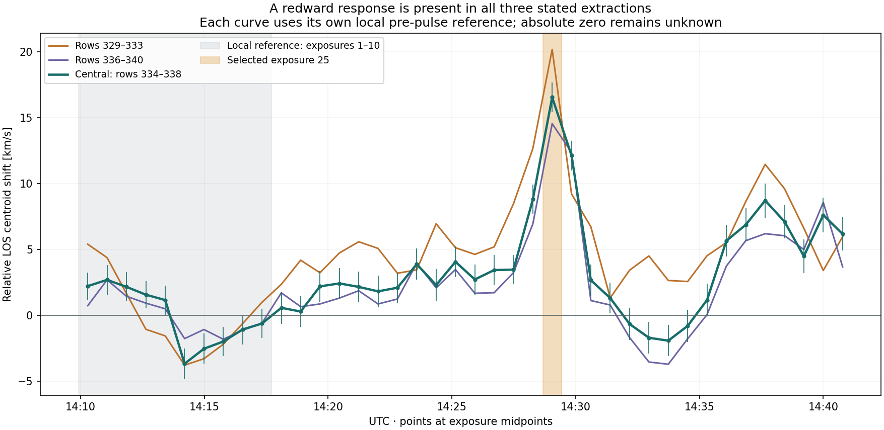
The same ten-exposure reference gives +14.6 to +20.2 km/s across the three stated spatial extractions. For the central extraction, changing the reference to its first or second five exposures gives +14.6 ± 1.2 or +18.5 ± 1.2 km/s.
These comparisons show why the small formal fit error is not the whole uncertainty. Across the three extractions and three reference choices, the values are +13.3 to +22.0 km/s. The redward sign remains in these tested choices. This is not a bound over all possible alignments, backgrounds or wavelength errors.
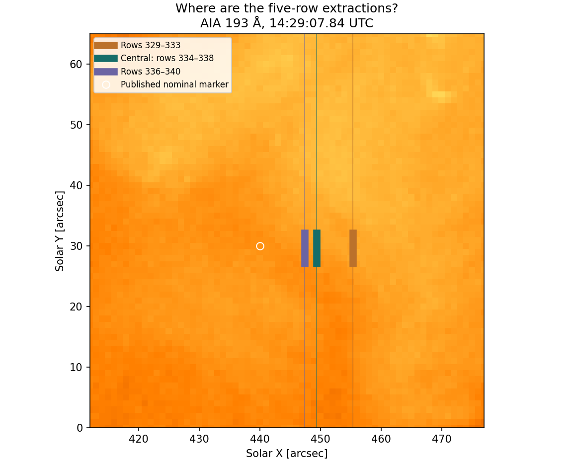
| Extraction | Rows (zero based) | Δx, Δy mapping | Relative shift at exposure 25 |
|---|---|---|---|
| Alternative A | 329–333 | +15″, -6″ | +20.2 ± 1.1 km/s (formal 1σ) |
| Central | 334–338 | +9″, -11″ | +16.6 ± 1.1 km/s (formal 1σ) |
| Alternative B | 336–340 | +7″, -13″ | +14.6 ± 1.1 km/s (formal 1σ) |
The central reference spans 14:09:55.000–14:17:42.289 UTC (exposures 1–10). The selected integration spans 14:28:40.646–14:29:25.646 UTC (exposure 25). We fit each of the five row spectra separately, then average their centroids with equal weights. We do not rebin or interpolate spectra before fitting.
The rows stay fixed on the detector. The slit pointing changes by a few arcseconds during the record, so this is not tracking one plasma parcel. The mapping alternatives are linked X/Y choices retained from the preceding spatial comparison; they are not independent error bars.
| Quantity | Value / range | Origin | Source / method | Uncertainty meaning | Use / limit |
|---|---|---|---|---|---|
| Event and feature | E05; 16 February 2011; first narrow redshift response near the previously selected crossing | SOURCE-DERIVED candidate + new local extraction | Veronig et al. (2011); R124–R126 | Exact source-paper spatial bin remains UNKNOWN. | New row selection is identified separately from the published measurement. |
| Central spatial extraction | Five fixed detector rows 334–338, zero based; nominally near y≈+30″ under the R126 candidate mapping | ANALYSIS CHOICE grounded in measured spatial structure | R126 Δx=+9″, Δy=−11″; processed EIS Fe XIII coordinates | Five rows give a 5″ sampling width; this is not ±2.5″ alignment accuracy. | Fit each native row separately and average the five centroids equally. |
| Alternative extractions | Rows 329–333 with mapping (+15″,−6″); rows 336–340 with mapping (+7″,−13″) | ANALYSIS CHOICES / mapping alternatives | Actual R126 region optima; paired X/Y choices retained | Overlapping samples, not independent detections or confidence bounds. | No rows were chosen to reproduce the published peak amplitude. |
| Selected integration | EIS exposure 25: 14:28:40.646–14:29:25.646 UTC, about 45 s | MEASURED metadata | Original counters and processed-header times checked in R125/R126 | Timestamp decimals reproduce saved precision, not clock accuracy. | The result averages an evolving scene over the integration. |
| Local reference | Same detector rows, mean centroid of exposures 1–10; 14:09:55–14:17:42 UTC | MEASURED spectra + ANALYSIS CHOICE | Saved processed EIS record and stated averaging rule | The reference is not assumed stationary. Its fit-noise contribution is propagated. | Relative temporal change only; not the publication’s quiet-Sun zero. |
| Relative line shift | +16.6 ± 1.1 km/s in the central extraction at exposure 25 | DERIVED HERE from measured spectra | Gaussian + linear background; archived wavelength correction | ±1.1 km/s is formal 1σ from fit/photon/read noise and reference mean only. Systematic and registration errors are not included. | Positive means redward relative to the chosen local reference. |
| Spatial-choice effect | +14.6 to +20.2 km/s using the same ten-exposure reference | DERIVED HERE / comparison of stated choices | Three fixed five-row extractions | Spread of these three results, not a bound over every possible alignment. | The redward sign remains in the tested extractions. |
| Time-reference effect | Central extraction: +14.6 ±1.2 km/s (exposures 1–5 reference); +18.5 ±1.2 km/s (6–10) | DERIVED HERE / comparison of stated choices | Two non-overlapping halves of the chosen pre-pulse interval | The reference centroids differ by about 3.9 km/s. This is not an absolute-zero calibration. | All three apertures × three reference choices give +13.3 to +22.0 km/s; this finite comparison is not a full uncertainty envelope. |
| Absolute Doppler zero | UNKNOWN | UNKNOWN | Source paper sets zero using quiet-Sun averages; exact mask/time range not recovered | Residual orbital correction, true background flow and absolute wavelength uncertainty are not bounded here. | Do not call +16.6 km/s an absolute plasma speed. |
| Normal plasma velocity and MHD type | UNKNOWN from this extraction alone | UNKNOWN | Need local front normal, projection, velocity reference and plasma-state constraints | No normal-flow, magnetic or compression prior inserted. | A redward spectral response is not a fast/slow classification. |
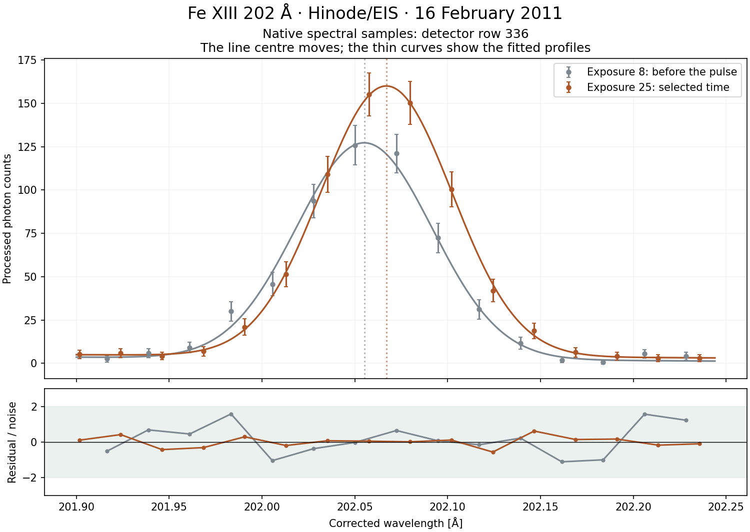
For each native row and time, corrected wavelength is the stored window wavelength minus the archived wave_corr. We follow the EISPAC reader convention. We fit the Fe XIII window over 201.900–202.244 Å using a Gaussian plus a linear background. Fitting uses processed photon counts, so no absolute radiometric conversion is needed for the relative centroid change.
Δv = c × (mean centroid at time t − mean reference centroid) / 202.044 Å.
The denominator sets the line’s velocity scale. It does not set the measured zero to a laboratory rest frame. Each mean gives equal weight to the same five detector rows; the reference then averages the first ten times.
Formal errors use the public EISPAC photon/read-noise prescription and local fit covariance. The reference contribution is propagated; points inside that reference include their covariance with the mean. Because all later points share a reference, their errors are correlated. Processing correlations, residual wavelength drift, line-model mismatch and spatial registration are outside this formal error.
For the next physical step: relate this relative line response to the same front patch and its local normal, while keeping the unknown background velocity explicit. It is not yet a normal plasma velocity or an upstream/downstream state pair. No RMO family calculation is performed here.
The update includes exact row selections, native spectral subsets, corrected wavelength arrays, fitted parameters/covariances, every fit-quality flag, reference comparisons, figures and viewer data. Earlier source files and results remain in the full project.
Result: a measured relative spectral response in an explicit extraction. Absolute velocity, normal flow and MHD family remain open.
E05 · 16 FEBRUARY 2011 · AIA / HINODE–EIS
Veronig et al. (2011) · Data and methods
Stable structures along the slit give a useful candidate alignment. The exact published Doppler bin still needs to be identified.
We compare Fe XII 195 Å structure from EIS with AIA 193 Å, following the established cross-instrument approach described by Pelouze et al. (2019). Here EIS kept its slit at one location. This provides less spatial information than a full raster.
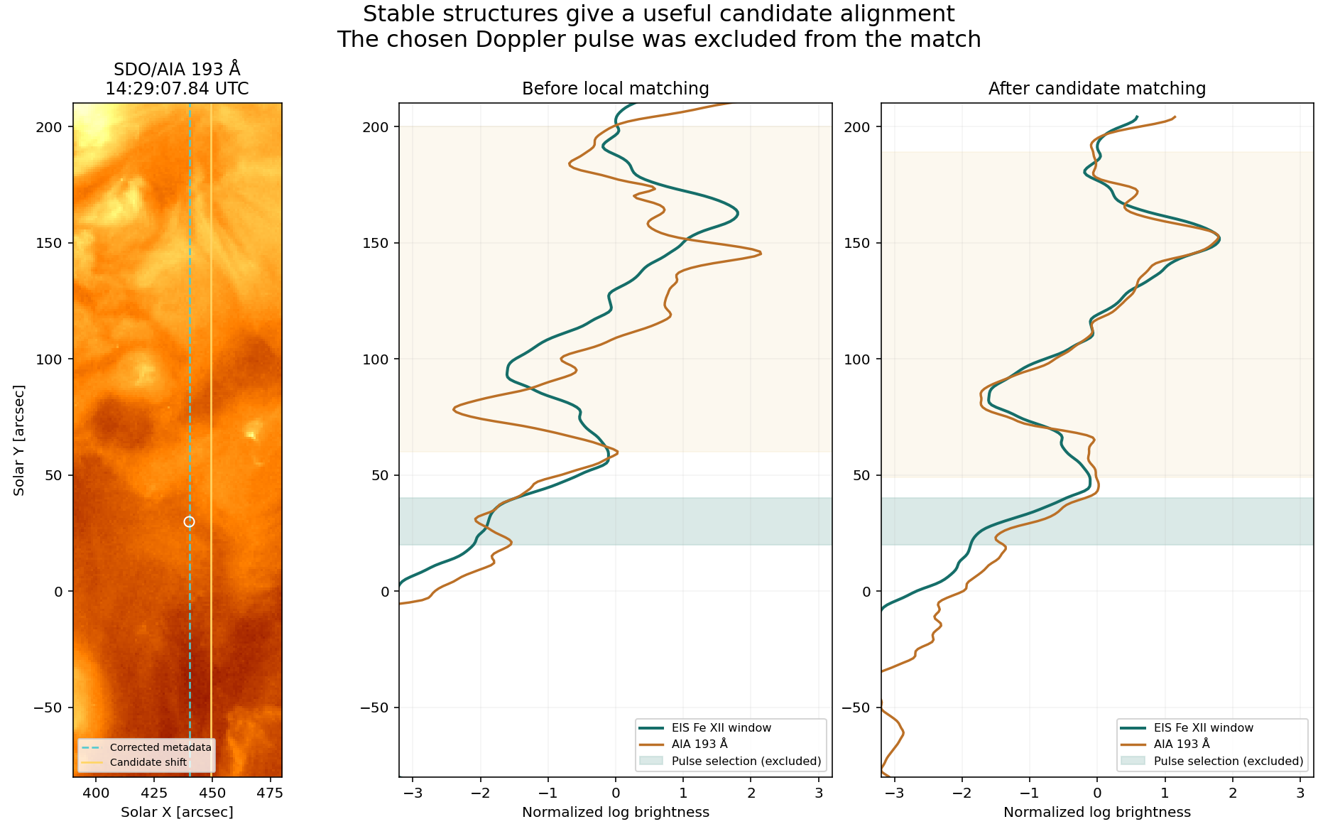
The similarity of spatial brightness profiles. We used the processed EIS spectrum and four native AIA images taken within its exposure.
Quiet-looking parts of the slit, a limited shift search and the same light spatial smoothing. Rows that changed by more than 10% across three EIS exposures were left out.
A reproducible candidate for the next spatial extraction. It does not yet establish the published bin, a normal plasma velocity or an MHD mode.
For the combined northern interval, the four images prefer +8″ to +9″ in X and −12″ to −11″ in Y. Those are fitted positions on a 1″ search grid. They are not a ±1″ error bar.
When separate structures are used, the best positions range from +7″ to +15″ in X and −13″ to −6″ in Y. The image comparison also has a broad ridge: different X and Y shifts can partly compensate each other. These facts keep the alignment provisional.
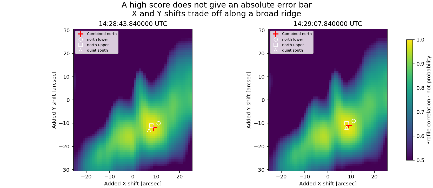
A high correlation means that the selected profiles have similar shapes. It does not prove that all of the emitting plasma is the same. AIA uses a broad wavelength band; EIS uses a narrow window. The scene evolves while EIS integrates for about 45 seconds. A single slit also leaves its roll angle poorly constrained.
Measured file metadata, published processing, our image-derived result and missing physical inputs are shown separately. No literature value was inserted to close a missing plasma input.
| Quantity | Value / range | Origin | Source / method | Uncertainty meaning | Use / limit |
|---|---|---|---|---|---|
| Event and candidate | 16 February 2011; E05; first narrow Fe XIII redshift pulse near published x=440″, y≈+30″ | SOURCE-DERIVED + analysis choice | Veronig et al. (2011), Figures 1–3; R124 candidate | The +20″ to +40″ selection is not ±10″ measurement error. | The published spatial extraction bin is not yet recovered. |
| Processed EIS record | eis_20110216_140955.data.h5 + .head.h5; exposure 25, array index 24 | SOURCE-DERIVED processing; MEASURED timing metadata | Official EISPAC/NRL level-1 archive through its NASA mirror | Header times agree with native counters within 0.000484 s rounding; this does not establish absolute clock accuracy. | Same TL_ID 21079, 40 exposures and native 2″ slit. EIS_PREP was not rerun here. |
| AIA comparison | Four 193 Å images; starts 14:28:43.84, 14:28:57.56, 14:29:07.84, 14:29:22.23 UTC | MEASURED image and exposure metadata | SDO/AIA level-1 files, VSO / JSOC / NSO delivery | Exposure lengths ≈2.000, 0.750, 2.000 and 0.263 s. All lie inside EIS exposure 25. | Compare each separately; four short images do not reproduce the full 45 s EIS integration. |
| Corrected nominal slit position | x≈440.398″ at exposure 25; Fe XII row coordinates include a 16.208-pixel CCD offset | SOURCE-DERIVED calibration + MEASURED pointing metadata | Per-exposure solar_x and stored offsets, following the EISPAC reader conventions | These are calibration inputs, not an independently measured absolute alignment error. | Use the time-dependent solar_x for this fixed-slit record; its 40 columns are time samples, not a spatial raster. |
| Candidate local translation | Δx≈+9″; Δy≈−11″; candidate slit x≈449.4″ | DERIVED HERE from observed spatial structure | EIS Fe XII 195 Å window and AIA 193 Å profile comparison | Representative candidate, NOT ±1″ accuracy and NOT a 1σ result. Absolute registration error remains UNKNOWN. | Add this translation to the corrected EIS coordinates. Do not replace the published slit coordinate without qualification. |
| Repeatability across four AIA times | Combined northern region: Δx=+8 to +9″; Δy=−12 to −11″ | DERIVED HERE; consistency comparison | Same EIS exposure and overlapping northern structures | Range of fitted optima on a 1″ grid, not independent confidence limits. | The preferred area repeats; nearby correlated X/Y alternatives remain. |
| Dependence on selected structures | Separate regions: Δx=+7 to +15″; Δy=−13 to −6″ | DERIVED HERE; analysis choices | Northern halves and a quieter southern segment | This observed spread is not a calibrated uncertainty envelope. Region limits and smoothing are choices. | A single rigid translation is still provisional; roll was not measured. |
| What the brightness comparison measures | Relative spatial structure in a 24-pixel Fe XII window and a broad AIA band | DERIVED HERE from processed images | Stored pre-flight conversion curve; normalized log profiles; equal 1.5″ Gaussian smoothing | Includes continuum / blends. No absolute radiometric error is inferred. | No Gaussian fit, line-ratio density, temperature or plasma velocity is obtained. |
| Fe XIII bin and Doppler reference | Exact published bin UNKNOWN; published response remains about +20 km/s relative to its quiet-Sun reference | SOURCE-DERIVED velocity; UNKNOWN native extraction | Veronig et al. (2011); R124–R125 | Selected fit error and absolute velocity reference remain UNKNOWN. | An illustrative raw row mapping is not the source bin; no velocity is assigned to it. |
| Normal flow and MHD family | UNKNOWN for an independently reconstructed local state pair | UNKNOWN | Need the same patch, justified normal and plasma-state constraints | No angle, flow or magnetic prior is inserted. | No new RMO calculation or family identification. |
The processed EIS pair matches the native programme and all 40 exposure times. The largest time difference is 0.000484 s, consistent with the stored millisecond rounding; durations differ by at most 0.00000381 s from the native values. These checks do not measure the absolute accuracy of the instrument clock.
| AIA start UTC | AIA end UTC | Exposure [s] | Inside EIS 25 |
|---|---|---|---|
| 14:28:43.840000 | 14:28:45.839677 | 1.999677 | Yes |
| 14:28:57.560000 | 14:28:58.310392 | 0.750392 | Yes |
| 14:29:07.840000 | 14:29:09.839675 | 1.999675 | Yes |
| 14:29:22.230000 | 14:29:22.492961 | 0.262961 | Yes |
The EIS metadata supplies +6.667″ and −2.470″ pointing corrections. The mean Fe XII CCD offset is 16.208 pixels. We follow the EISPAC coordinate conventions, using per-exposure solar_x for this fixed-slit sequence. This gives nominal x≈440.398″ at exposure 25 before our local image comparison.
The earlier R125 raw-reference estimate and these processed coordinates use different correction conventions. Their numerical difference is not an independently measured error. The stored calibration offsets are not counted as a second independent confirmation of our image match.
The four AIA comparisons share the same EIS exposure and many structures. They check consistency, but they are not four independent statistical detections. We do not turn their scatter into a confidence interval.
Still missing: the actual published Fe XIII extraction bin, its velocity reference and the local front-normal geometry. Under the candidate translation, a raw Fe XIII row near 336 would map near y=+30″. That illustrative mapping is not proof that this is the published bin, and we attach no Doppler value to it.
aia__lev1:193:1076941759, 1076941772, 1076941783, 1076941796.The saved update includes six source files (about 67 MB), query and download records, hashes, processed profiles, image grids, score maps, figures, code and the input table.
Result: useful candidate alignment; exact source bin and normal flow remain open. Earlier event results and model tests remain available.
E05 · 16 FEBRUARY 2011 · AIA / HINODE–EIS
Veronig et al. (2011) · Source paper · Data and methods
Two AIA images were taken while EIS was collecting the candidate spectrum. The next question is whether they sample the same place on the front.
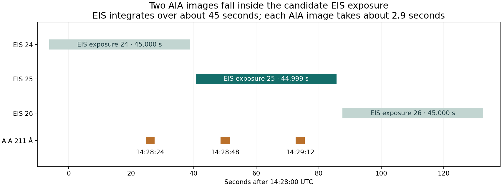
One original EIS file and three AIA 211 Å images. We read their times, exposure lengths and pointing information, then compared their integration intervals.
The spectrum averages about 45 seconds of an evolving scene. An AIA image takes about 2.9 seconds. Their time labels should not be treated as three instantaneous measurements of one plasma state.
A small difference remains between the nominal slit coordinates. We have not measured the image-alignment correction or linked a raw detector bin to the published Doppler pulse.
The circle marks the candidate chosen from the published figures. The two lines show the published slit position and a nominal position from the native metadata. They help us see what still needs to be aligned.
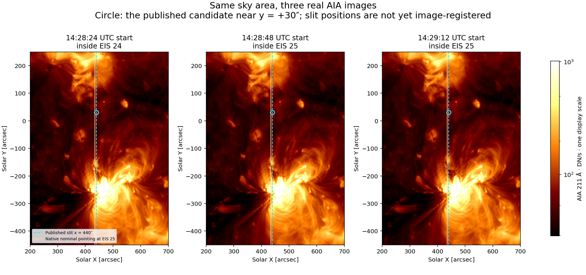
Here we subtract images taken 24 seconds apart. Bright and dark patches can help locate movement. These differences do not give a density jump or an MHD mode.
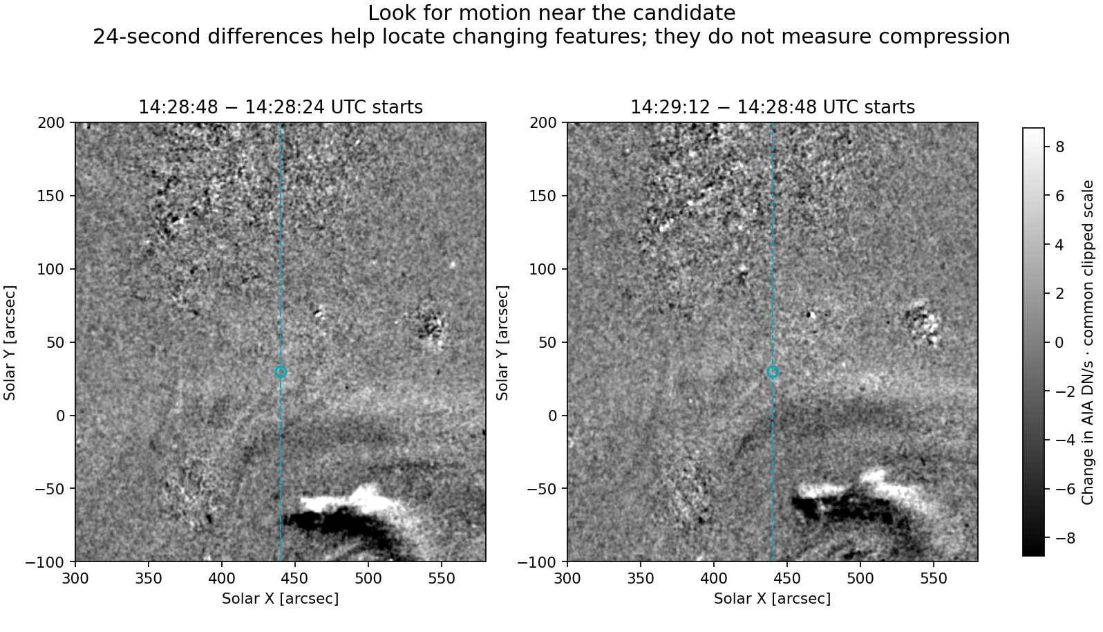
Measured metadata comes from the instrument files. Source-derived values come from a published analysis or a stated calibration. Our selection of a candidate is an analysis choice. Missing physical inputs remain unknown.
| Quantity | Value | Origin | Source / method | Uncertainty meaning | Use / limit |
|---|---|---|---|---|---|
| Event and selected feature | 16 February 2011; first narrow Fe XIII redshift pulse near x=440″, y≈+30″ | Source-derived + analysis choice | Veronig et al. (2011), Figures 1–3; selection retained from R124 | No error assigned to the figure reading. The +20″ to +40″ interval is a selection window, not ±10″ measurement error. | The exact published processed bin is still to be recovered. |
| EIS candidate exposure | 25th exposure (array index 24): 14:28:40.646–14:29:25.646 UTC; duration 44.999459 s | Measured metadata; timing derived from counters | Native EIS FITS + SolarSoft time conversion | Decimals reproduce counters, not measured clock accuracy. Absolute clock uncertainty is not established here. | Contains both selected AIA images at 14:28:48 and 14:29:12. |
| AIA reference image | 211 Å; starts 14:28:48.620 UTC, ends 14:28:51.521 UTC | Measured metadata | Native AIA FITS from VSO/JSOC; EXPTIME=2.901247 s | Actual exposure interval, not a ± error bar or a 12 s integration. | Fully inside EIS exposure 25 under the recorded clock convention. |
| Second AIA image | Starts 14:29:12.620 UTC, ends 14:29:15.521 UTC | Measured metadata | Native AIA FITS; EXPTIME=2.901248 s | Same timing qualification. Selected images are 24 s apart; this is not a claim that the instrument cadence was 24 s. | Also inside EIS exposure 25. |
| Earlier AIA image | Starts 14:28:24.620 UTC, ends 14:28:27.521 UTC | Measured metadata | Native AIA FITS; EXPTIME=2.901249 s | Same timing qualification. | Inside EIS exposure 24, not 25. |
| Native EIS sampling | 2″ slit; 40 exposures; start-to-start spacing 46.852–47.104 s; about 45 s integration | Measured metadata | SLIT_ID, NEXP, TI1 and MHC_DUR in the selected file | Range across this record, not a statistical uncertainty. | The paper gives nominal 1″ and 49 s programme values. Keep both descriptions visible; do not silently use the nominal values as native metadata. |
| Slit position | Published x=440″. Header reference plus relative pointing gives x≈434.73″ at the candidate exposure. | Source-derived coordinates + measured pointing metadata | Paper; CRVAL1 and relative XCEN_TI1 change | Separation ≈5.27″ is not a measured shift, error bar or 1σ value. No absolute alignment bound is available. | Spatial registration remains open. No shift is fitted to force the signals to agree. |
| EIS detector row | Exact processed row/bin UNKNOWN | Unknown | Header-linear candidate is around row 323 (zero based); details below | Wavelength-dependent Y correction, spatial binning and residual alignment remain unresolved. | The published +20 km/s is not assigned to this raw row. |
| Doppler response | About +20 km/s relative to the source quiet-Sun reference | Source-derived | Veronig et al. (2011), Figure 3; R124 reading | Selected line-fit uncertainty and absolute reference offset UNKNOWN. | No new spectral fit; no normal plasma velocity inferred. |
| Local normal, normal flow and local jump-frame speed | UNKNOWN | Unknown | Need the same patch, a front-surface model and a justified projection | No angle or flow bound is assumed. | Time overlap alone does not close these inputs. |
| Compression, paired temperature and coronal vector field | UNKNOWN for the selected patch | Unknown | No new density, DEM or magnetic inversion | No literature prior inserted in this stage. | No new MHD family is identified. |
EIS exposure 25 starts at 14:28:40.646484 and ends at 14:29:25.645943 UTC. These decimals reproduce the saved counters. They do not establish microsecond clock accuracy. The earlier published pulse time is an approximate figure reading.
| AIA exposure start UTC | Exposure end UTC | Duration [s] | Inside EIS exposure |
|---|---|---|---|
| 14:28:24.620000 | 14:28:27.521249 | 2.901249 | 24 |
| 14:28:48.620000 | 14:28:51.521247 | 2.901247 | 25 |
| 14:29:12.620000 | 14:29:15.521248 | 2.901248 | 25 |
We follow the public SolarSoft convention: interpret TI1 as an unsigned counter, use 1/512-second steps relative to OBT_TIME, and anchor the result to DATE_OBS. The integration length is MHC_DUR / 10⁶, following eis_data::getexp. The separate TI2 interval is recorded, but is not substituted for the measured integration length.
For AIA, the interval is DATE-OBS to DATE-OBS + EXPTIME. Its T_OBS is close to the midpoint. The one-second interval returned by a catalogue query is not the camera exposure.
The paper places the slit at x=440″. The native first-exposure coordinate reference is x=432.427″; the relative pointing change at exposure 25 is about +2.304″. Their sum is about 434.73″. The remaining 5.27″ separation is a difference between two coordinate descriptions. It is not an independently measured image shift.
The native file reports a 2″ slit and roughly 47-second sampling; the publication describes nominal 1″ and 49-second values. This is a metadata/reduction detail to reconcile for the selected record. It does not by itself revise the published physical interpretation.
A simple linear reading of the header puts y≈+30″ near zero-based row 323. A real Fe XIII extraction also needs the wavelength-dependent spatial correction, the actual bin definition and local image registration. We therefore do not attach the published Doppler value to that raw row.
A calibrated slit intensity profile and a suitable AIA image comparison are needed to constrain the offset. For this check we retain the nominal overlay and leave the registration error unknown. No local 3D front normal or normal plasma flow is inferred.
nan string. These cards and the source bytes are retained unchanged; the full image arrays were checked separately.Timing is now tied to native files. The exact processed spatial bin, residual registration, velocity reference and local normal remain the limits on a physical flow inference.
eis_l0_20110216_140955.fits.gz.aia__lev1:211:1076941740, 1076941764, 1076941788. Original bytes, queries, delivery URLs and SHA-256 checksums are saved.The update includes the input table, all 40 EIS exposure records, the three native AIA files, the original EIS file, common-grid image arrays, figures and scripts. The public source note for the 2017 JPEG viewer is simplified; the exact original filenames and supplied-source history remain in the processing records.
Result: native time overlap checked; spatial registration remains open. The earlier model checks, event results and image viewers remain available.
E05 · 16 FEBRUARY 2011 · AIA + HINODE/EIS
The spectrum adds a real plasma constraint: a redshift pulse of about 20 km/s. To use it in RMO, we still need to connect that line-of-sight component to the local front normal.
Veronig et al. (2011), Figure 1; RMO composite with an approximate reading of Figure 3. View original source
A propagating EUV feature and a co-located redshift response. One selected published profile has a pulse of about +20 km/s relative to the chosen quiet-Sun zero.
The first narrow pulse near nominal y ≈ +30″ on the x = 440″ slit, with the AIA 211 Å display at 14:28:48 UT as image context. This is a figure-level candidate, not a verified detector aperture.
Spectroscopy adds a component of plasma motion. It is physically different from the motion of the bright pattern. A normal-frame state pair has not yet been established.
Exact time overlap, spectral fit error and zero reference, local 3D normal, density jump, temperature and magnetic state. No new fast, slow, rotational or contact identification is made.
First resolve the EIS exposure and detector row, then the nearby AIA frame headers and local image registration. This checks whether the two signals describe the same passage before any normal-flow inference.
The published start speeds near 590 km/s come from global propagation fits along an assumed spherical solar surface. They are not the front speed at our selected instant, nor a reconstructed 3D normal speed. The approximately 20 km/s value is a line shift relative to a quiet-Sun reference. The two measurements use different directions, averages and definitions.
The relevant quantity for a local jump is w = V_front,n − u_n: front motion and plasma motion along the same normal, at the same place and time, in a consistent reference frame.
Let ℓ point away from us, so redshift is positive. Let n be the unit front normal, and split the plasma velocity into a normal part and a tangential part: u = u_n n + u_t.
v_D + v_ref = u · ℓ = u_n (n · ℓ) + u_t · ℓ
The published Doppler zero removes a quiet-Sun reference, represented here by v_ref. It does not establish zero upstream flow. Moreover, a fitted optically thin line is emission-weighted; relating it to one local fluid velocity requires an emitting-component assumption.
Only if tangential motion is set to zero, the reference is known and n · ℓ ≠ 0 can we write u_n = (v_D + v_ref)/(n · ℓ). That is a conditional deprojection, not an automatic correction. Near a normal perpendicular to the line of sight, it becomes ill-conditioned. With unconstrained tangential motion, one LOS component generally does not determine normal flow.
No angle or flow prior is inserted in this table. The later goal is to quantify what a justified geometry model permits, while retaining its assumptions.
All numerical source values below are source-derived. This stage did not reduce new telescope data. Our chosen location is an analysis choice. Unknowns stay unfilled; a quoted instrument capability is not a measured error for our selected sample.
| Quantity | Value / range | Origin and method | Uncertainty meaning | Association and use |
|---|---|---|---|---|
| Event and feature | 16 February 2011; first narrow Fe XIII redshift pulse | SOURCE-DERIVED · Veronig et al. (2011), arXiv:1111.3505, pp. 6–8, Figures 1–3 | Event identity; no numerical uncertainty assigned | Northward passage along EIS slit; later redshift lane and ejecta are separate → Defines the candidate feature |
| Candidate position | x = 440″; nominal y ≈ +30″; selection interval y = +20″ to +40″ | ASSUMED / analysis choice · This work: choose one stacked profile in Figure 3; source slit x on p. 8 | Selection interval, not a coordinate error, detector bin or 1σ range | Figure-level candidate only; actual detector row and registration error unknown → Locate a candidate for a later header/registration check |
| AIA reference image | 211 Å; displayed time 14:28:48 UT; ratio denominator 14:23:36 UT | SOURCE-DERIVED · Veronig et al. (2011), arXiv:1111.3505, Figure 1, upper right | Displayed labels; exact integration interval not recovered | Plausible context for the selected EIS pulse; simultaneous exposure overlap not certified → Visual association; not a density jump |
| Selected EIS pulse time | About 14:28:40 UT | SOURCE-DERIVED · This work: read the red marker of the nominal +30″ profile in Figure 3 | Approximate figure reading; no physical timing bound or 1σ error assigned | About 7 s before the AIA image label; this alone does not certify an exposure match → Candidate time, not a native timestamp |
| Selected Doppler response | About +20 km/s; positive = redshift | SOURCE-DERIVED · This work: Figure 3 reading, consistent with source peak scale; single-Gaussian line method on p. 6 | Selected-fit uncertainty UNKNOWN; symbol dimensions are not error bars | Quiet-Sun-relative, emission-weighted line shift; not yet a local upstream/downstream velocity pair → LOS plasma observable; not normal flow |
| EIS sampling | 45 s integration + 4 s readout; nominal 49 s cadence | SOURCE-DERIVED · Veronig et al. (2011), arXiv:1111.3505, Methods, pp. 5–6 | Instrument/programme context; actual exposure start/end and timestamp convention UNKNOWN | One time label can represent an extended integration → Needed to test time overlap and phase |
| AIA sampling | Nominal cadence up to 12 s; 0.6″ pixels; about 1.5″ resolution | SOURCE-DERIVED · Veronig et al. (2011), arXiv:1111.3505, Methods, p. 6 | Nominal sampling, not a position error or selected-frame exposure duration | Exact selected frame headers not recovered → Context only |
| Doppler zero and uncertainty | Quiet-Sun mean used as zero; local fit error and absolute reference offset UNKNOWN | SOURCE-DERIVED · Veronig et al. (2011), arXiv:1111.3505, Methods, pp. 5–6 | The stated better-than-±5 km/s capability is not the selected-pixel error or a 1σ bound | Reference-region choice and line-of-sight mixtures may affect a bulk-flow interpretation → Do not treat the relative zero as u₁,n = 0 |
| Local normal front speed | UNKNOWN at the selected time | UNKNOWN · A new local track and a specified front surface would be needed | No numerical interval assigned | Published global fit starts and mean speeds are not the local normal speed → Required with normal plasma flow for a frame transformation |
| Local front normal / projection | UNKNOWN in 3D; no new image-normal fit performed | UNKNOWN · Selected front patch, height and geometry are not reconstructed here | No angle prior or deprojection factor adopted | A surface propagation direction need not be the normal to a 3D dome → Needed to relate LOS flow and front motion to the same normal |
| Compression X = ρ₂/ρ₁ | UNKNOWN; no significant jump established for this candidate | UNKNOWN · Veronig et al. (2011), arXiv:1111.3505, pp. 7–10; Figures 2 and 5 | Small expected density changes lie within the reported diagnostic noise; this does not measure X = 1 | The prominent density lane is delayed and associated with the eruption behind the front → Do not import that lane or an intensity-based guess as a measured shock jump |
| Temperature / thermal pressure | UNKNOWN as a paired local state | UNKNOWN · Veronig et al. (2011), arXiv:1111.3505, line diagnostics, pp. 8–11 | Formation temperatures around 1.2–2.5 MK are response context, not a measured temperature interval | No matched upstream/downstream temperature or total pressure established → A closure and a joint thermal state would be needed |
| Magnetic field and its jump | UNKNOWN | UNKNOWN · No independent coronal vector pair extracted in this stage | No field-strength or angle prior adopted | No same-patch B₁, B₂ or characteristic-speed constraint → Fast/slow/Alfvénic or rotational-jump tests remain incomplete |
| Normal plasma velocity / frame speed | u₁,n, u₂,n and w = V_front,n − u_n: UNKNOWN | UNKNOWN · Projection and reference equations below | No valid numerical bound from one relative LOS component alone | Requires consistent place, phase, velocity reference and front normal → Not ready for a two-state RMO calculation |
Both tracks use distance along the assumed spherical surface from x = 440″, y = −267″. The earlier circular-front centre was fitted at x = 462 ± 29″, y = −267 ± 21″. This geometric construction does not determine the normal to a 3D front.
| Track | Quantity | Published value | Source |
|---|---|---|---|
| AIA 211 front | Initial quadratic-fit speed | 585 ± 56 km/s | Veronig et al. (2011), arXiv:1111.3505, pp. 8–9, Figure 4a |
| AIA 211 front | Quadratic acceleration | −675 ± 160 m/s² | Veronig et al. (2011), arXiv:1111.3505, pp. 8–9, Figure 4a |
| AIA 211 front | Linear-fit mean speed | 336 ± 15 km/s | Veronig et al. (2011), arXiv:1111.3505, pp. 8–9, Figure 4a |
| EIS Fe XIII peak positions | Initial quadratic-fit speed | 587 ± 50 km/s | Veronig et al. (2011), arXiv:1111.3505, p. 9, Figure 4a |
| EIS Fe XIII peak positions | Quadratic acceleration | −539 ± 48 m/s² | Veronig et al. (2011), arXiv:1111.3505, p. 9, Figure 4a |
| EIS Fe XIII peak positions | Linear-fit mean speed | 371 ± 12 km/s | Veronig et al. (2011), arXiv:1111.3505, p. 9, Figure 4a |
Reported ± fit errors. Sigma convention, parameter covariance and exact fit-reference epoch have not been recovered; no confidence level is assigned here.
Do not use a start speed as the local speed near 14:28:40 UT. Do not apply an additional image deprojection to these surface-distance fits. Different propagation sectors have different fitted speeds; their values are not transferred to this crossing.
The publication derives densities from the Fe XIII 202/203 Å line ratio. The prominent enhanced-density lane occurs behind the leading pulse, with a delay of about 100–150 s and different intensity/flow behaviour. The authors associate it with the eruption. It cannot be assigned to the selected leading front.
The reported intensity enhancement can suggest a small density increase only under fixed-temperature and emitting-volume assumptions. The expected change is within the density diagnostic noise. Thus neither X ≈ 1.1 nor X = 1 is entered as a measured jump.
Intensity maxima tend to follow Doppler maxima by about one EIS step. A shifted correlation is not a simultaneous upstream/downstream pair. Velocity, intensity and density from the same spectra also share calibration and line-of-sight dependencies; they are not independent replicas of one constraint.
Veronig et al. (2011), primary paper · ApJL 743, L10 · DOI 10.1088/2041-8205/743/1/L10. Methods and results: source PDF pp. 5–11; Figures 1–5. The plot is a publication-based visual aid.
Veronig et al. (2011), Figure 3, lower panel. View original source
The saved script reads the PDF vector curve and marker for one nominal profile. Its exact rendering coordinates are retained for reproducibility. The displayed time and amplitude are rounded. Marker size is graphical detail, not a timing or spectral-fit uncertainty. PDF polyline vertices are not a native exposure table.
No extra spectral fit, raw-image registration, DEM, MHD solve or robustness sweep was performed. The original source PDF, source hash, candidate selection, table and script are retained in the checkpoint.
Resolve one EIS observation and its exposure/row metadata around this passage, together with a small set of AIA 211 Å frame headers. Check the time convention and local registration before estimating a projected normal. This is a targeted matching step, not a new full-event reduction or solver run.
The earlier twelve-record catalogue, E11 results, logo and image viewers remain available in QuickLook. R124 adds this input table; it does not revise the completed E11 conclusions.
Twelve selected records now share one input-and-result index. The completed E11 analysis remains bounded and ambiguous. Other publications supply different useful constraints; none is promoted here to a newly identified solar mode.
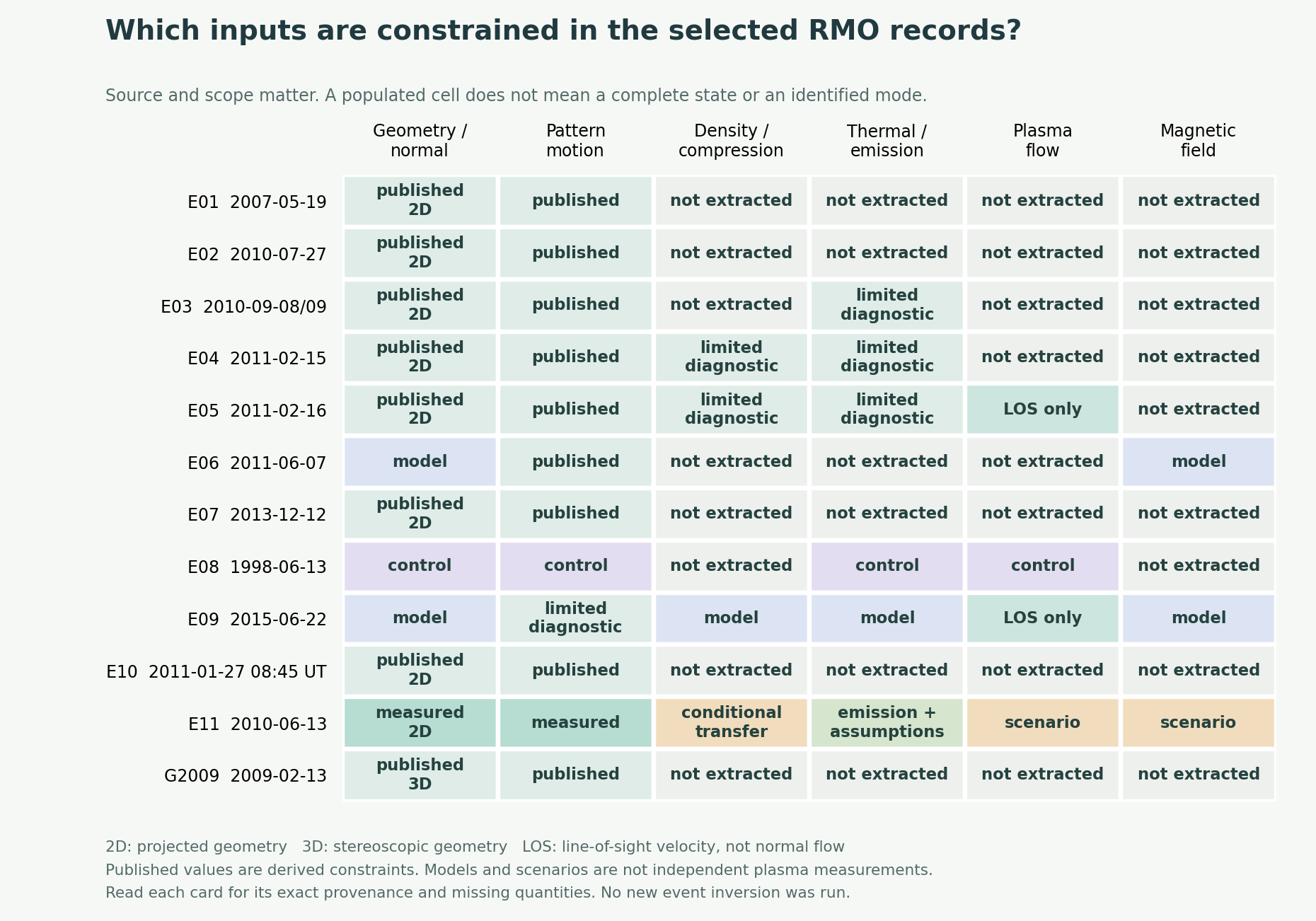
| Code | Meaning |
|---|---|
| — | No usable constraint extracted here; not a claim that no data exist. |
| D | Published derived constraint; not necessarily complete. |
| D2 | Published projected geometry; local 3D normal not established. |
| D3 | Published stereoscopic geometry; not a full plasma state. |
| DM | Model-derived information; not a measured local vector or state jump. |
| D* | Published diagnostic with a specific limitation; read the card. |
| DLOS | Published line-of-sight flow; not normal flow. |
| M | Retained RMO measurements. |
| M2 | Retained projected geometry and conditional normal. |
| MD* | Retained measured emission plus conditional thermal information. |
| CD | Published diagnostic transferred only under stated association assumptions. |
| C | Accepted instrument/association control. |
| A | Conditional scenario; the local observed state is unknown. |
| Record / date | RMO result at this checkpoint | Most useful missing constraint |
|---|---|---|
| E01 · 2007-05-19 | Published speed comparison retained. It demonstrates a measurement-definition issue, not an RMO family identification. | A matched front track at a defined cadence; then same-patch plasma-frame information. |
| E02 · 2010-07-27 | Two-feature literature case retained. The trailing feature is not independently identified as a slow MHD wave. | Same-feature motion relative to plasma, with local geometry. |
| E03 · 2010-09-08/09 | Identity resolved. Published propagation evidence is useful; no new two-sided MHD classification is made. | A selected train/front patch with an independent local characteristic-speed or plasma-state constraint. |
| E04 · 2011-02-15 | Suitable for a bounded thermodynamic consistency comparison. A density estimate is conditional on the emission model. | The line-of-sight/emitting-volume constraint, followed by the local plasma and magnetic state. |
| E05 · 2011-02-16 | Best next publication-based test of pattern motion versus plasma motion. No family is selected by this triage. | The projection relating the measured LOS velocity to local normal flow at the crossing. |
| E06 · 2011-06-07 | A useful geometry/model-field case; a complete measured state pair is not supplied by the retained summary. | Independent local field/state constraints and uncertainty in the model normal. |
| E07 · 2013-12-12 | A partially constrained kinematic case. Missing plasma inputs remain unknown. | Same-patch plasma-frame and thermodynamic constraints. |
| E08 · 1998-06-13 | CONTROL ONLY. The accepted audit is retained; a spectral null does not establish an absent wave or exclude a family. | No new measurement requested: preserve the existing control scope. |
| E09 · 2015-06-22 | Related flare-loop benchmark, not an independently reproduced RMO result or a global EUV-front identification. | A closure-compatible observed/model state comparison with explicit provenance. |
| E10 · 2011-01-27 08:45 UT | A valid kinematic example; flare class and catalogue speed cannot identify a jump family. | Local geometry and plasma-frame information for one specified epoch. |
| E11 · 2010-06-13 | R119 outer bounds retained. The R120–R122 inner block is complete with mode unresolved: F1 slow is conditional; actual fast, Alfvénic or material-boundary alternatives are not excluded. | Independent same-patch normal plasma flow, then the joint field/thermal state. |
| G2009 · 2009-02-13 | The published geometry comparison is reproduced in saved RMO work. It is not a full MHD inversion. | Independent local plasma and field information, if a mode claim is intended. |
Fast, slow, Alfvénic and material-boundary explanations require different measurable relations. Missing magnetic data can leave a test open; they do not select or exclude a family. Any feasible-state search must use the same declared constraints for competing explanations, rather than tune unknowns toward a desired answer.
| Explanation | What would test it? | What we must not infer |
|---|---|---|
| Fast or slow compressive wave / shock | Normal speed relative to plasma, local characteristic speeds, and two-sided compression/pressure/field constraints. | For a shock, conservation and admissibility must also hold. Slower image motion is not a slow-mode label. |
| Alfvén wave / rotational discontinuity | Correlated transverse velocity and field-direction changes; for an ideal RD, constant density, thermal pressure and field magnitude, with Alfvénic propagation. | An intensity movie alone cannot test these coupled conditions. A failed fixed-state example is not a solar exclusion. |
| Contact / tangential material boundary | Normal motion with the plasma: zero mass flux through the boundary, plus the appropriate pressure/field jump conditions. | A moving bright edge is not automatically a material boundary; LOS velocity alone does not establish normal advection. |
| Intermediate shocks / degenerate limits / compound structures | The relevant jump solution, characteristic structure, closure and admissibility. | Not interchangeable with an Alfvénic RD. Incomplete solver coverage is not evidence of physical absence. |
| CME structure / changing emission / line-of-sight superposition | Feature identity, plasma motion, channel/spectral response and geometry over time. | An apparent front need not be a single MHD discontinuity. Overtaking alone does not choose between these explanations. |
The normal plasma-frame speed is w = V_front,n − u_n. A magnetogram measures the photospheric field; a coronal model can supply conditional geometry but does not directly measure a coronal field jump. A field inferred by assuming a fast shock cannot then serve as independent proof of that shock type. See the ideal-MHD jump conditions and oblique-shock relations.
Publication interpretation: A propagating EUV disturbance has channel- and cadence-dependent measured kinematics.
RMO result: Published speed comparison retained. It demonstrates a measurement-definition issue, not an RMO family identification.
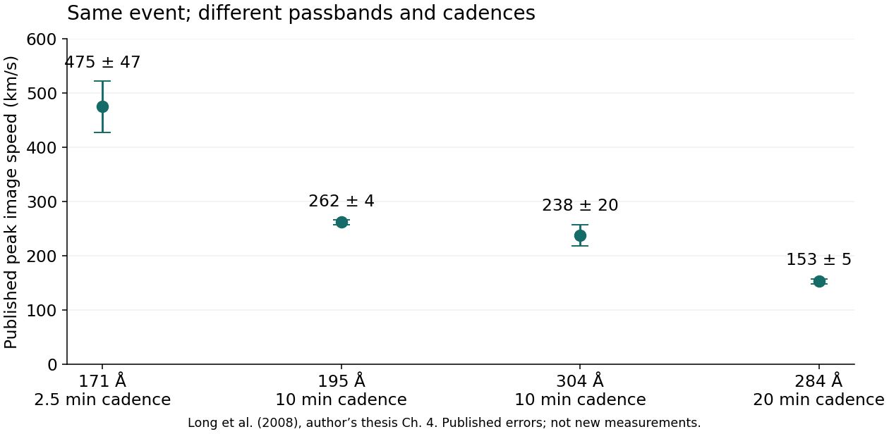
| Quantity | Value / range | Origin | Uncertainty meaning | Association / dependency |
|---|---|---|---|---|
| Peak image speeds: 171 / 195 / 304 / 284 Å | 475 ± 47 / 262 ± 4 / 238 ± 20 / 153 ± 5 km/s | SOURCE-DERIVED | Reported fit uncertainties; statistical definition not re-established here. | Cadences 150 / 600 / 600 / 1200 s. These are not four coeval fluid speeds. |
| Local normal, plasma flow, state jumps | Not supplied by these speed rows | UNKNOWN | Not bounded | A front track is not a two-sided plasma state. |
What is missing: A matched front track at a defined cadence; then same-patch plasma-frame information.
A useful bounded question: Select one channel/feature/time definition before any branch comparison.
Primary source · Long: thesis Chapter 4, Table 4.1; Long et al. 2008, doi:10.1086/589742
Reading status: Retained source extraction; no repeat raw reduction.
Publication interpretation: The authors interpret the leading feature as a fast wave and the trailing feature through field-line stretching.
RMO result: Two-feature literature case retained. The trailing feature is not independently identified as a slow MHD wave.
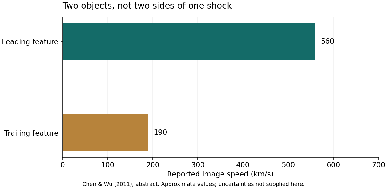
| Quantity | Value / range | Origin | Uncertainty meaning | Association / dependency |
|---|---|---|---|---|
| Leading / trailing pattern speed | about 560 / 190 km/s | SOURCE-DERIVED | Approximate published values, not uncertainty intervals. | Distinct image features; no measured shared upstream state. |
| Normal flow and magnetic/thermal jumps | Not recovered | UNKNOWN | Not bounded | Do not assign a mode from the speed ordering. |
What is missing: Same-feature motion relative to plasma, with local geometry.
A useful bounded question: Keep the two feature tracks and their origins separate.
Primary source · Chen & Wu 2011, abstract; doi:10.1088/2041-8205/732/2/L20
Reading status: Retained source extraction.
Publication interpretation: The authors interpret the global disturbance and quasi-periodic trains as fast-mode waves.
RMO result: Identity resolved. Published propagation evidence is useful; no new two-sided MHD classification is made.
Liu et al. (2012), Figure 4. View original source
| Quantity | Value / range | Origin | Uncertainty meaning | Association / dependency |
|---|---|---|---|---|
| Event identity | 8–9 September 2010 | SOURCE-DERIVED | Date confirmed from the primary timeline. | The eruption begins on 8 September; observations cross midnight. |
| Front propagation | Published direction- and height-dependent tracks | SOURCE-DERIVED | Use the uncertainty of each selected track, not one global speed. | Figures 3–5; the CME flank is a separate feature. |
| Thermal signature | Channel changes are reported | SOURCE-DERIVED | Not a recovered local temperature/density pair. | EUV response and line-of-sight mixture remain dependencies. |
What is missing: A selected train/front patch with an independent local characteristic-speed or plasma-state constraint.
A useful bounded question: Choose one published cut and separate its wave track from the CME flank.
Primary source · Liu et al. 2012, Table 1 and Figures 1, 3–5; doi:10.1088/0004-637X/753/1/52
Reading status: Primary PDF timeline, methods and figure passages inspected in R123.
Publication interpretation: A weakly compressive, thermally changing EUV disturbance is analysed.
RMO result: Suitable for a bounded thermodynamic consistency comparison. A density estimate is conditional on the emission model.
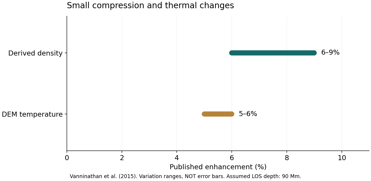
| Quantity | Value / range | Origin | Uncertainty meaning | Association / dependency |
|---|---|---|---|---|
| Density enhancement | 6–9% | SOURCE-DERIVED | Reported enhancement range; not a confidence interval. | DEM/EM conversion assumes a line-of-sight depth of 90 Mm. |
| Electron-temperature enhancement | 5–6% | SOURCE-DERIVED | Reported enhancement range; not an independent error box. | Temperature and emission measure come from the same inversion. |
| LOS depth | 90 Mm | ASSUMED | Source modelling assumption, not a measured error bound. | Density depends on depth and filling factor; electron temperature is not total pressure. |
What is missing: The line-of-sight/emitting-volume constraint, followed by the local plasma and magnetic state.
A useful bounded question: Carry the density–temperature dependencies into one chosen patch; do not use an independent rectangular error box.
Primary source · Vanninathan et al. 2015, methods/results; doi:10.1088/0004-637X/812/2/173
Reading status: Retained primary extraction.
Publication interpretation: The paper interprets the correlated EUV and Doppler response as plasma pushed downward by a coronal wave.
RMO result: Best next publication-based test of pattern motion versus plasma motion. No family is selected by this triage.
Veronig et al. (2011), Figure 1. View original source
| Quantity | Value / range | Origin | Uncertainty meaning | Association / dependency |
|---|---|---|---|---|
| Initial speed along the slit / deceleration | 590 km/s / −540 m/s² | SOURCE-DERIVED | Published fit values; complete covariance not extracted. | Pattern motion along a slit is not local normal propagation. |
| Line-of-sight plasma response | Redshift up to 20 km/s; later blueshift about −5 km/s | SOURCE-DERIVED | Extrema, not ± errors; line-fit/systematic uncertainty must accompany any selected sample. | EIS coronal lines; compare the same slit position and exposure with AIA. |
| Density diagnostic | Fe XIII 202/203 Å; wave compression not securely resolved above noise | SOURCE-DERIVED | A limited diagnostic, not a measured zero jump. | A non-detection cannot supply X = 1. |
| Normal plasma velocity and field change | Not determined by LOS velocity alone | UNKNOWN | Not bounded | Requires a geometry constraint or an explicitly conditional projection. |
What is missing: The projection relating the measured LOS velocity to local normal flow at the crossing.
A useful bounded question: Make one matched AIA/EIS crossing table, with exposure timing, geometry and spectral uncertainties. Stop before an RMO solve.
Primary source · Veronig et al. 2011, observations, diagnostics and Figures 1–5; doi:10.1088/2041-8205/743/1/L10
Reading status: Primary PDF diagnostic and figure passages inspected in R123.
Publication interpretation: CASHeW characterizes the coronal bright front and its model magnetic environment.
RMO result: A useful geometry/model-field case; a complete measured state pair is not supplied by the retained summary.
Source figures and instrument details are available in the linked publication. The shared matrix shows which inputs this card currently constrains.
| Quantity | Value / range | Origin | Uncertainty meaning | Association / dependency |
|---|---|---|---|---|
| Radial front speed | Maximum about 1200; mean about 800 km/s | SOURCE-DERIVED | Summary values, not simultaneous states or error bounds. | Front, peak and back have distinct tracks. |
| Field direction / shock geometry | PFSS and front-model information | SOURCE-DERIVED | Model-dependent; local uncertainty not transcribed. | An HMI-constrained PFSS field is not a measured coronal vector jump. |
What is missing: Independent local field/state constraints and uncertainty in the model normal.
A useful bounded question: Select one front point and label every PFSS-derived quantity as model-derived.
Primary source · Kozarev et al. 2017, Section 3.1 and Figure 4; doi:10.1051/swsc/2017028
Reading status: Retained primary methods/results extraction.
Publication interpretation: An off-limb bright front is characterized.
RMO result: A partially constrained kinematic case. Missing plasma inputs remain unknown.
Source figures and instrument details are available in the linked publication. The shared matrix shows which inputs this card currently constrains.
| Quantity | Value / range | Origin | Uncertainty meaning | Association / dependency |
|---|---|---|---|---|
| Mean radial front speed | about 450 km/s | SOURCE-DERIVED | Approximate mean; no error distribution recovered. | C4.6-associated eruption; flare class does not define an MHD family. |
| Co-spatial thermodynamic and vector states | Not extracted | UNKNOWN | Not bounded | Pipeline capabilities must not be treated as numbers measured for this patch. |
What is missing: Same-patch plasma-frame and thermodynamic constraints.
A useful bounded question: Audit one published front track and the diagnostics actually reported for it.
Primary source · Kozarev et al. 2017, Section 3.2; doi:10.1051/swsc/2017028
Reading status: Retained primary results extraction.
Publication interpretation: The source study distinguishes the moving components and revisits their spectral interpretation.
RMO result: CONTROL ONLY. The accepted audit is retained; a spectral null does not establish an absent wave or exclude a family.
Source figures and instrument details are available in the linked publication. The shared matrix shows which inputs this card currently constrains.
| Quantity | Value / range | Origin | Uncertainty meaning | Association / dependency |
|---|---|---|---|---|
| Outer front versus erupting filament | Separate objects in the accepted audit | SOURCE-DERIVED | Instrument-conditioned limits retained. | TRACE/EIT/CDS/SUMER; this is not an IRIS event. |
| SUMER response / Mg X interpretation | Null wave response and O IV blend caveat retained | SOURCE-DERIVED | Sensitivity, cadence and line blending limit interpretation. | Do not transfer the filament spectrum to the weak outer front. |
What is missing: No new measurement requested: preserve the existing control scope.
A useful bounded question: Use this as an association and instrument-sensitivity control, without reopening its audit.
Primary source · Madjarska et al. 2015; Harra & Sterling 2003; accepted project audit; doi:10.1051/0004-6361/201424754
Reading status: Retained accepted control, not rerun.
Publication interpretation: The authors identify propagating slow shocks through conductive MHD modelling and spectral comparisons.
RMO result: Related flare-loop benchmark, not an independently reproduced RMO result or a global EUV-front identification.
Ye et al. (2026), Figure 4; model panels a–h and observed panels i–l. View original source
| Quantity | Value / range | Origin | Uncertainty meaning | Association / dependency |
|---|---|---|---|---|
| Observed spectra and morphology | IRIS Fe XXI and AIA/SJI comparison | SOURCE-DERIVED | Profile uncertainties must be recovered for a numerical test. | Figure 4 i–l are observations; a–h are model results. |
| Shock speeds, jumps and local field | Model quantities in the proposed interpretation | SOURCE-DERIVED | Not an observed upstream/downstream state pair. | Do not import the synthetic compression or component speeds as measurements. |
| Energy treatment | Conductive, nearly isothermal shocks in the model | SOURCE-DERIVED | Physical closure, not an observational error. | Changing gamma alone is not a demonstrated match to the RMO energy equation. |
What is missing: A closure-compatible observed/model state comparison with explicit provenance.
A useful bounded question: Check the energy-flux treatment before any adiabatic RMO comparison.
Primary source · Ye et al. 2026, Figures 4–6 and thermal-conduction discussion; doi:10.1038/s41467-026-75039-z
Reading status: Primary article and figure passages inspected in R123.
Publication interpretation: Published EUV-front kinematics include this B-class-associated event.
RMO result: A valid kinematic example; flare class and catalogue speed cannot identify a jump family.
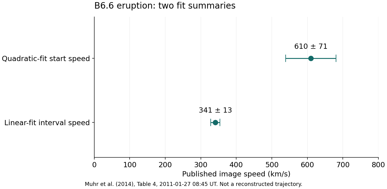
| Quantity | Value / range | Origin | Uncertainty meaning | Association / dependency |
|---|---|---|---|---|
| Linear speed / quadratic initial speed / acceleration | 341 ± 13 km/s / 610 ± 71 km/s / −340 ± 48 m/s² | SOURCE-DERIVED | Published fit uncertainties; no covariance or sigma convention inferred here. | The 08:45 UT B6.6 row only; do not mix the other events on the same day. |
| Normal, plasma flow, temperature and magnetic state | Not supplied by that catalogue row | UNKNOWN | Not bounded | The linear and initial quadratic speeds are different estimands. |
What is missing: Local geometry and plasma-frame information for one specified epoch.
A useful bounded question: Choose a speed definition and retain the original fit interval before using the row.
Primary source · Muhr et al. 2014, Table 4; doi:10.1007/s11207-014-0594-7
Reading status: Retained primary table extraction.
Publication interpretation: Published EUV and radio interpretations provide conditional constraints on the outer front.
RMO result: R119 outer bounds retained. The R120–R122 inner block is complete with mode unresolved: F1 slow is conditional; actual fast, Alfvénic or material-boundary alternatives are not excluded.
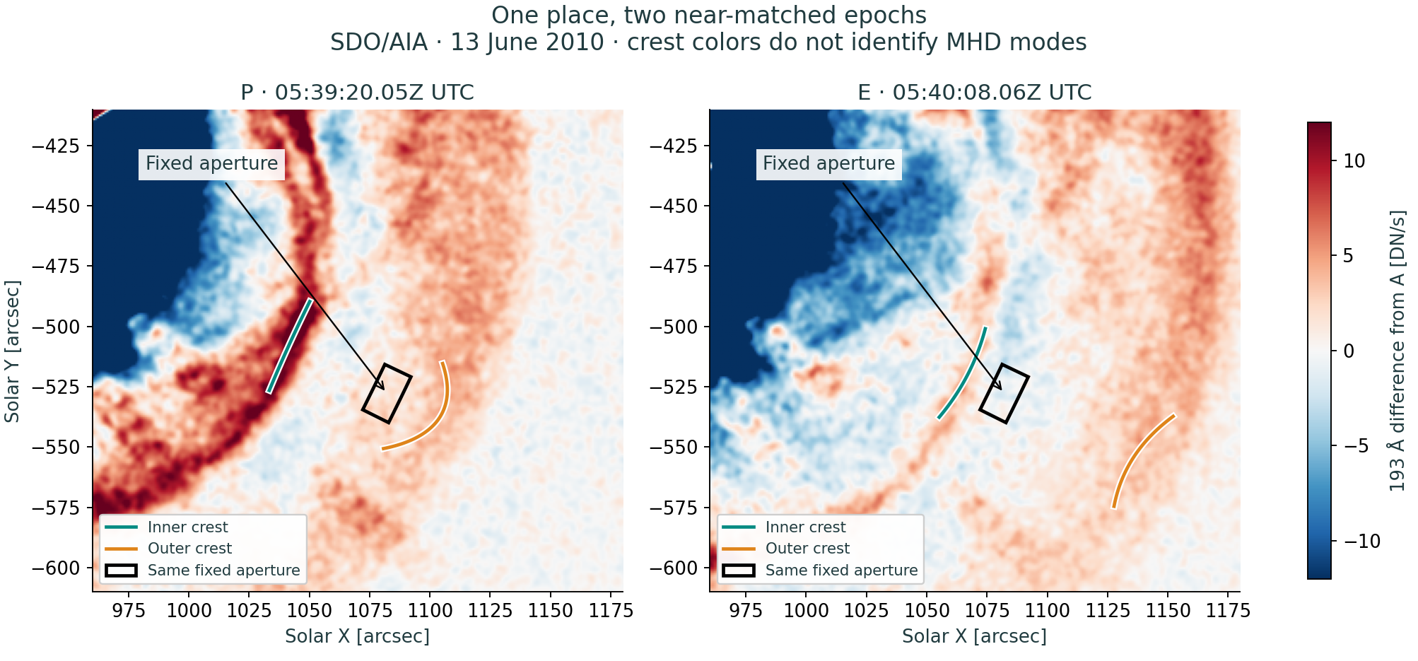
| Quantity | Value / range | Origin | Uncertainty meaning | Association / dependency |
|---|---|---|---|---|
| Matched 96 s inner / outer image rates | 409.1 / 687.5 km/s | MEASURED / RMO saved reduction | Method ranges about 397.9–417.7 / 686.2–784.5 km/s; not complete errors. | Image tracks do not provide plasma normal flow. |
| Outer radio density and compression | Conditional radio-derived inputs retained from R108–R119 | SOURCE-DERIVED | Lane ranges are hard scenarios; frequency inputs are dependent. | Emission-harmonic, split-lane and same-patch association assumptions are explicit; not transferred to the inner front. |
| Interfront 171/193/211 changes | Measured channel changes retained from R122 | MEASURED / RMO saved reduction | Mask/reference envelopes, not 1σ or complete systematics. | A fixed-aperture time series is not a jump across the inner front. |
| Intermediate flow, field and thermodynamic jump | Unknown; P/F1/F2 are conditional completions | ASSUMED | No observed error range for these states. | F1 supports a checked slow solution only if its unmeasured state is adopted. |
What is missing: Independent same-patch normal plasma flow, then the joint field/thermal state.
A useful bounded question: Reopen only when a concrete independent state or jump constraint becomes available.
Primary source · Project R119–R122 saved reports and their source receipts are controlling; Ma et al. 2011 is one input source.
Reading status: Completed project evidence retained, not recomputed.
Publication interpretation: Stereoscopy changes the inferred surface-pattern speed for the selected front patch.
RMO result: The published geometry comparison is reproduced in saved RMO work. It is not a full MHD inversion.
| Quantity | Value / range | Origin | Uncertainty meaning | Association / dependency |
|---|---|---|---|---|
| Surface-pattern speed: apparent / corrected | about 260 / 207 km/s | SOURCE-DERIVED | Three matched table comparisons, not one error bar. | Tables 4–5; 05:45–05:55 UT, sectors 18–19. Same-patch association already accepted. |
| Local magnetic/plasma state pair | Not determined by the geometry tables | UNKNOWN | Not bounded | Do not replace missing 3D vectors/covariance with scalar height rows. |
What is missing: Independent local plasma and field information, if a mode claim is intended.
A useful bounded question: Retain as the worked geometry example; no repeated geometry audit.
Primary source · T. Podladchikova et al. 2019, Tables 4–5; doi:10.3847/1538-4357/ab1b3a
Reading status: Accepted geometry result retained.
E03 is the 8–9 September 2010 wave-train study, published in 2012. The overtaking sharp fronts are in Liu et al. (2010), 8 April 2010, published in ApJL 723, L53–L59 and deposited on arXiv in 2012. This separate reference is saved as a reserve, without silently changing the twelve-record pool.
Two different image speeds, or one front passing another, do not by themselves establish a fast–slow pair. We would first need to identify the tracked features and the plasma state each one encounters.
Use the published 16 February 2011 observations to make one matched crossing table: slit position, front location, exposure times, image-pattern speed, LOS velocity and line-fit uncertainties. Identify the projection information required to obtain normal plasma flow. Leave unsupported quantities unknown and stop before an RMO solve.
This case adds a plasma observable distinct from pattern motion. It is selected for that diagnostic value, not because it promises a fast, slow, Alfvénic or contact result. The overtaking Liu event remains an interesting subsequent two-feature case; E09 needs a conductive-versus-adiabatic closure comparison before a numerical RMO benchmark.
The saved model checks and the bounded E11 work are sufficient to begin the next input-table stage. No additional generic robustness sweep is needed for that task. A new numerical claim would still require its own input, closure and admissibility checks.
The principal bottlenecks are local normal flow, field strength and direction on the relevant sides, emitting-volume assumptions in density inference, and a demonstrated match between instruments and features. This is a physical prioritization, not a computed information-gain ranking. Literature values may define explicit scenarios; typical values are not automatically justified uncertainty bounds.
R123 is a catalogue triage. No new FITS, spectral reduction, DEM inversion, RMO solve or mode identification. New source checks: E03 identity, E05 diagnostics, E09 model/observation and closure distinction, and the separate overtaking-front reference. Earlier source extractions and completed controls are retained as such.
RMO · check a new observational constraint
Two image tracks and changing emission are established. The inner MHD mode remains unresolved; the F1 slow solution is conditional.
E11 · 13 June 2010 · R122 combined observational result. Two moving image features are retained from R120. New measurements show changing emission in one fixed region between them. The actual MHD identity of the inner feature remains unresolved. The checked F1 slow-shock solution is conditional; it is not a solar identification or a preferred interpretation.
| Question | Answer |
|---|---|
| What did we measure? | Two image tracks in the earlier stage; now exposure-normalized AIA signals in the same fixed image aperture at near-matched times. |
| What changed? | At the two primary epochs, 211 Å is brighter than the early reference by about 28–34%, while 171 Å is fainter. A small 193 Å increase becomes a decrease. The signs persist across the declared aperture and reference choices. |
| What did we assume? | Retained pointing calibration; an image aperture selected from the crest geometry; limited temporal transfer of that geometry. F1 additionally assumes a particular intermediate plasma state produced by an outer fast jump. |
| What does RMO say? | F1 supplies a valid conditional inner slow jump. Existing observations do not independently establish that F1 is the actual plasma entering the inner front. Other physical explanations remain open. |
| What remains ambiguous? | Density/compression, temperature, normal plasma flow, vector magnetic field, line-of-sight mixing and whether the image ridge marks a discontinuity. |
| What should be measured next? | Prioritize the plasma velocity along the inner-front normal in the same region and epoch. It gives the relative propagation speed and tests a material boundary. Magnetic and thermodynamic information would still be needed to distinguish wave families. |
The primary aperture is the annular sector at projected solar radius 1198–1210 arcsec, position angle 115.5–116.5 degrees. Here position angle is computed as atan2(solar X, solar Y), modulo 360 degrees, in the retained image coordinates. Its centre is 1204 arcsec, PA 116 degrees. It was declared before the new photometry. This is an image aperture, not an isolated emitting volume or a tracked fluid parcel.
The two main epochs are P and E. D and L show later evolution only: the inner crest is arriving at, or has crossed, this region. They are not certified samples of plasma between the fronts.
| Group | 193 Å UTC | 171 Å UTC | 211 Å UTC | Interpretation |
|---|---|---|---|---|
| P | 05:39:20.05 | 05:39:24.55 | 05:39:26.05 | Primary interfront sample |
| E | 05:40:08.06 | 05:40:12.55 | 05:40:14.06 | Primary interfront sample |
| D | 05:40:32.05 | 05:40:36.55 | 05:40:38.06 | Inner arrival / later context |
| L | 05:41:08.07 | 05:41:12.57 | 05:41:14.07 | Later context |
The channels differ by up to 6.01 seconds. Intensities are not interpolated to manufacture simultaneous measurements. For the image-location check only, the inner crest is interpolated between adjacent retained 193 Å tracks. Continuing outward motion of the outer crest during the small channel delay is assumed. For the largest aperture, the inner clearance at the latest primary channel time is about 5.0 arcsec. The central outer curve stays outside that aperture by at least 11.5 arcsec at P and 44.3 arcsec at E. These checks do not bound all pointing, registration or three-dimensional errors.
The displayed difference images reuse the earlier image grid and use Gaussian smoothing of 1.2 arcsec for display. The numerical photometry below uses unsmoothed native detector pixels.
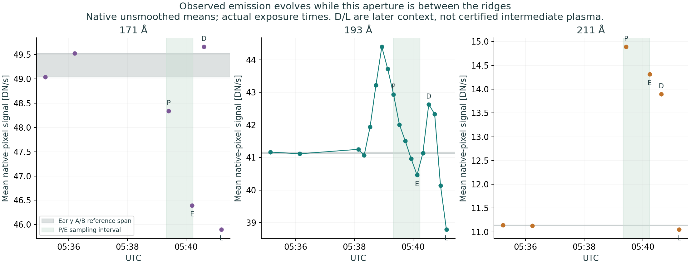
For each channel and aperture, the measured mean is the mean detector signal divided by exposure time, in DN/s. The reported change is 100 × (signal − reference) / reference. Reference A is near 05:35 and B near 05:36, using the retained exposure of each channel. They are early references, not independently certified undisturbed plasma.
| Epoch | Channel | Primary mean [DN/s] | Range over masks/references | Sign |
|---|---|---|---|---|
| P | 171 Å | 48.339 | -2.9% to -1.4% | negative all |
| P | 193 Å | 42.938 | +4.1% to +5.1% | positive all |
| P | 211 Å | 14.890 | +32.4% to +34.1% | positive all |
| E | 171 Å | 46.394 | -6.8% to -5.0% | negative all |
| E | 193 Å | 40.465 | -2.0% to -0.9% | negative all |
| E | 211 Å | 14.317 | +27.7% to +29.1% | positive all |
The ranges combine nine masks and two early references. All masks have the same centre; radial half-widths are 4, 6 and 8 arcsec and angular half-widths are 0.4, 0.5 and 0.6 degrees. These are explicit method/reference ranges, not total measurement errors, confidence intervals or 1σ. Spatial variation among pixels is saved separately and is not an error on the mean. The shared references, overlapping masks and channels are not independent evidence for density.
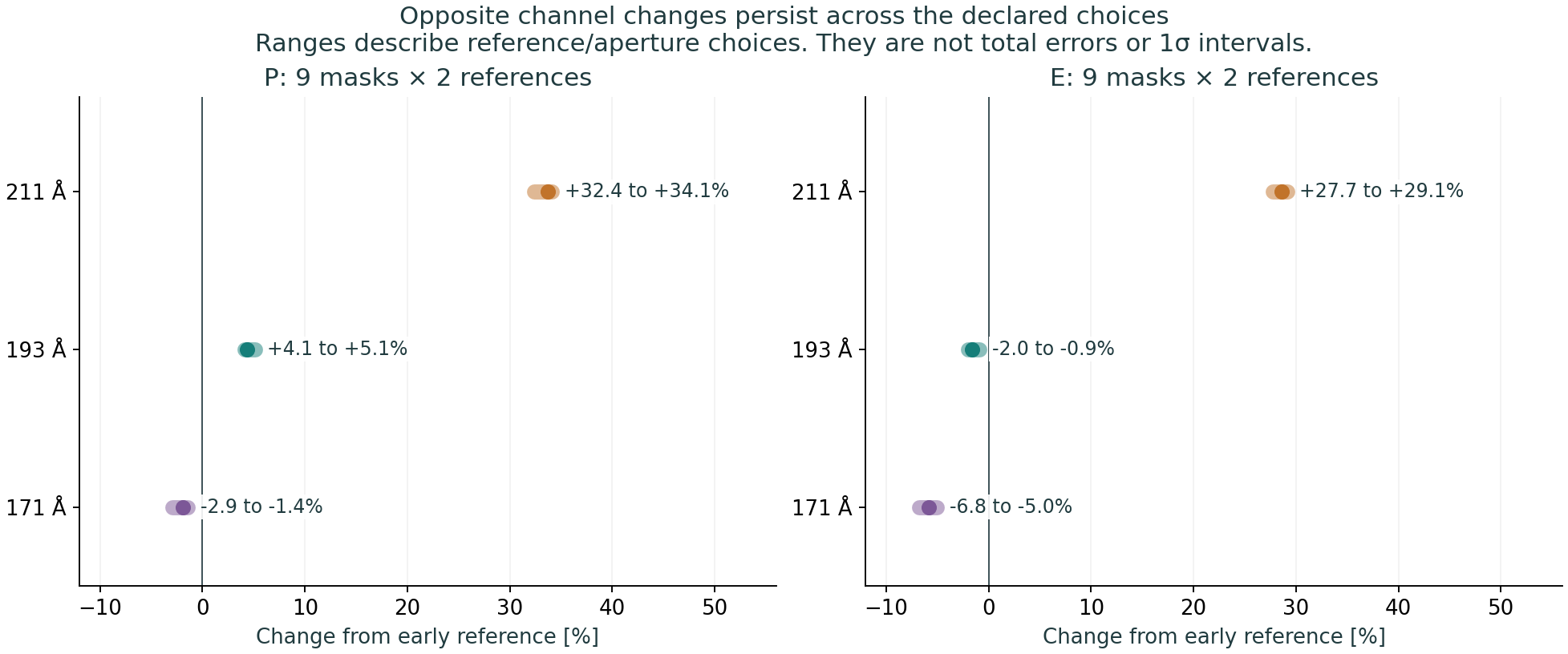
The 193 Å sequence is more densely sampled than 171 and 211 Å. No extra thermal information is created by connecting points. In particular, the later 171 Å sample D changes sign across the choices; the strong primary P/E statement must not be extended to every later epoch.
| Quantity | Value or status | Provenance | Meaning and limit |
|---|---|---|---|
| Detector signal and exposure | 30 retained FITS in 171/193/211 Å; all source hashes checked | MEASURED · SDO/AIA | No new FITS downloaded. QUALITY=0 and MISSVALS=0 in these files do not establish zero systematic error. |
| Image pointing | Retained R113 calibration and FITS metadata | SOURCE-DERIVED | Applied to native-pixel mask selection; no new full level-1.5 processing or PSF correction. |
| Aperture and two references | Explicit dimensions and times above | ANALYSIS CHOICE | Chosen before photometry; nine masks/two references bound only these choices. |
| Local apparent speeds | Matched 96-second tracks: inner 409.1 km/s; outer 687.5 km/s | DERIVED FROM EVENT IMAGES · R120 | Method ranges: inner 397.9–417.7; outer 686.2–784.5 km/s. Pattern speeds, not plasma velocities or full uncertainty bounds. |
| Inner normal geometry | Image-plane endpoint normal PA 117.52 degrees; G0 effective normal pattern speed 408.97 km/s | DERIVED GEOMETRY plus ASSUMED G0 projection · R120 | A mean track rate and an endpoint normal do not measure the instantaneous 3D normal speed. |
| Intermediate F1 state | ne≈8.44×10⁷ cm⁻³; T≈2.863 MK; total B≈2.370 G; inner normal flow≈253.70 km/s for azimuth 90 degrees | ASSUMED / MODEL-DERIVED · R110/R120 | Outer-downstream state transferred unchanged to the inner upstream; not an independent local measurement. |
| Radio density/compression | Earlier source constraints retained | SOURCE-DERIVED with CONDITIONAL spatial association | Radio lanes have not been imaged onto this aperture. Density and compression from those lanes share information. They are not inner-jump measurements. |
| Local intermediate temperature and density | UNKNOWN as independent physical state | No accepted inversion here | Channel counts and published unregistered/per-channel fits do not supply a unique joint Te/ne state. |
| Local normal plasma velocity and vector B | UNKNOWN | No same-patch independent constraint established in this bounded study | Central model values cannot be promoted to measurements. |
| Inner density and field jumps | UNKNOWN | No registered before/after fluid-state pair | Temporal brightening in a fixed aperture is not a density jump across the inner front. |
The published-source audit in R121 remains applicable. A field estimate ahead of the outer front is not a measurement between the fronts; a shock-derived temperature is not independent confirmation of a shock calculation. The emission analysis of Lee et al. (2019) has relevant phase information but no registered joint state for this new aperture. Ma et al. (2011) and Gopalswamy et al. (2012) retain their explicit model and spatial-transfer restrictions.
We kept the previously declared P/F1/F2 intermediate-state scenarios and three magnetic azimuth examples. We did not adjust unknown inputs to make a preferred family pass. The following table separates a test in those nine fixed scenarios from a statement about the Sun.
| Interpretation | Physical requirements | Fixed P/F1/F2 result | Observational outcome | Missing evidence / limit |
|---|---|---|---|---|
| Fast shock | Compression and entropy increase; super-fast upstream inflow; full RH and characteristic transition; tangential field grows in the regular oblique branch. | Necessary inflow condition fails in all nine fixed intermediate scenarios. No new shock solve. | NOT IDENTIFIED / NOT EXCLUDED for the actual Sun | Actual intermediate B, pressure, flow and inner jump are unknown. Different actual states can admit a fast disturbance. |
| Slow shock | Compression and entropy increase; slow characteristic crossed below normal Alfven speed; tangential field decreases; full RH. | Three saved F1 azimuth examples have a complete checked slow jump. P/F2 do not in this saved root set. | CONDITIONALLY COMPATIBLE; NOT IDENTIFIED | F1 is not independently selected. Emission changes do not supply its B, flow or density jump. |
| Alfvenic wave / rotational discontinuity | In ideal isotropic MHD, normal propagation relative to plasma is ±cAn. A finite RD preserves density, pressure and field magnitude, with linked tangential field/velocity rotation. | Necessary ∣w1∣=cAn equality fails in all nine fixed scenarios. This failure depends on their unmeasured states. | NOT IDENTIFIED / NOT EXCLUDED for the actual Sun | No vector field/velocity rotation or thermodynamic jump measurement. A bright projected ridge alone cannot test an RD. |
| Contact discontinuity | No normal mass flux relative to the boundary. In the ordinary Bn≠0 contact, pressure, velocity and field are continuous; density may change. | w1 is nonzero in all nine fixed scenarios, so an ordinary contact at the measured speed fails that closure. | NOT IDENTIFIED / NOT EXCLUDED for the actual Sun | The actual plasma normal speed is unknown. Image motion need not equal material motion. |
| Tangential discontinuity | No normal mass flux; Bn=0; continuous total pressure. Tangential field/flow and density can differ. | Nonzero w1 already fails the necessary material-boundary condition in the fixed scenarios. | NOT IDENTIFIED / NOT EXCLUDED for the actual Sun | No normal field or total-pressure balance measurement. A CME-related boundary is not automatically a measured tangential discontinuity. |
| Smooth fast or slow wave | A continuous perturbation; identify plasma-frame speed and correlated thermodynamic/field changes. Linear phase speeds are cf or cs. | Exact linear phase-speed equalities fail at the nine fixed central states. This is not a test of every nonlinear smooth wave. | UNRESOLVED | No measured fluid-state profiles or amplitude-dependent evolution; a projected ridge does not establish a discontinuity. |
| Intermediate shocks and switch limits | Intermediate shocks are distinct from incompressible RDs. Field reversal, limiting geometry, RH and admissibility require their own treatment. | The R120 retained nonsingular compressive roots supply only F1 slow solutions. No complete intermediate/switch-limit domain audit is claimed. | NOT TESTED COMPLETELY; NOT AUTOMATICALLY EXCLUDED | Finite root cutoffs and classifier coverage do not certify every degenerate/nonregular case. |
| Compound structure / full Riemann fan | Connecting states and all intervening waves must satisfy one initial-value problem. | The local two-jump construction does not solve a full fan. | NOT DETERMINED | The required initial and intermediate vector states are absent. |
The characteristic and jump requirements follow the ideal-MHD conservation relations and the oblique-shock relations. Here an RD means the ideal isotropic-MHD rotational discontinuity; the more general anisotropic relation discussed by Blagau et al. (2015) is not an extra measured constraint for E11. An intermediate compressive shock must not be silently equated with an incompressible RD.
The numerical equality tolerance used in the fixed-state screens is 10⁻⁶ km/s. It is an arithmetic tolerance, not the precision of the solar velocity measurement. Failure of an equality at an assumed central state does not exclude that family over unknown solar states. The retained compressive-root enumeration covers its declared nonsingular interval and cutoffs; it does not certify every switch limit, intermediate shock or full wave fan.
In the saved F1 central azimuth-90-degree example, the inner-front relative inflow is 155.27 km/s and the compression is 1.2965. The upstream slow speed is 128.53 km/s and normal Alfvén speed is 281.89 km/s. Downstream, the normal inflow is 119.76 km/s, below the downstream slow speed of 141.93 km/s. The tangential magnetic field decreases and the entropy change is positive. The earlier independent conservation and RMO checks agreed.
Those are saved model results, not a new solver run. The earlier 108/108 F1 method/azimuth combinations passed the slow test under that shared-state closure. This count is neither an observational probability nor proof that F1 is correct. The present emission measurements do not select F1, reject it formally, or turn it into an observationally favoured branch.
| Explanation | Outcome | Reason / limit |
|---|---|---|
| CME-related surface, compression or evolving structure | Retained observational alternative | Two ridges are measured; no independent material-surface or local jump diagnosis. CME morphology and MHD family are different questions. |
| Changing temperature, ionization, LOS mixture or geometry | Retained emission explanations | Opposite channel changes require more than a naive brightness-to-density conversion. The data do not distinguish these processes. |
| One scalar emission-measure change with fixed temperature/ion fractions, fixed response, fixed LOS geometry and static additive foreground | Point-estimate sign pattern inconsistent with this restrictive model | For positive channel responses, ΔI_i=G_i ΔEM has one sign in every channel. Near-matched samples have opposing signs under every declared mask/reference choice. Full instrument, timing and background systematics are not bounded, so this is a conditional consistency screen, not a statistical exclusion. |
One restricted hypothesis can be screened directly: with fixed temperature, ion fractions, channel response, line-of-sight geometry and a static additive foreground, a single scalar emission-measure change gives ΔIᵢ = Gᵢ ΔEM, where each response Gᵢ is positive. It predicts the same sign in every channel. The primary point estimates have opposite signs for every declared mask/reference choice.
This is a conditional consistency screen. The frames are not simultaneous and the complete noise, calibration, background and timing budget is not bounded. It is not a statistical rejection of every density-change model. Changes in temperature, ionization or line-of-sight mixture can alter the channel pattern. No unique temperature, density or compression follows from the signs alone. The gap time series is also not a state-jump measurement with which to reject an RD.
We therefore do not fit a unique Te/ne here. A meaningful emission constraint would require a justified common response/ionization and foreground model for a spatially matched sequence, with its uncertainties. Assigning a temperature because 211 Å brightens would overstate the data.
The bounded inner-front block is complete with an unresolved solar mode. The two image features and the new channel changes are the observational result. The F1 slow jump is a conditional model completion. Fast, Alfvénic, material-boundary and evolving-emission explanations have been considered; no claim of equal probabilities or exhaustive testing of all degenerate MHD solutions is made.
The outer-front conclusion from R119 is retained with its own conditional radio/temperature/geometry bounds. It must not be transferred to the inner front. Two ridges do not by themselves establish a fast–slow pair, two fast shocks, two CMEs, or a global magnetized blast solution.
The most useful next physical constraint in this construction is the same-patch normal plasma flow. It separates a material boundary from relative propagation and sets w = Vfront,n − uplasma,n. It will not identify fast versus slow without magnetic and thermodynamic information. At the limb, a Doppler line-of-sight velocity alone is not that normal flow; a justified projection reconstruction is required. This priority is a physical judgment, not a computed global information-gain ranking.
No automatic new robustness sequence follows. Reopen this inner-front identification only when a concrete independent local-state/jump constraint or a justified new emission model/data set can test a specific claim.
The catalogue assessment applies the same physical and provenance checks to each selected observational record. Each gets the same provenance and spatial/temporal association audit, a visual, an uncertainty statement, a map of surviving explanations where justified, and one explicit outcome. Missing data remain missing. Old completed checks are reused unless a specific claim exposes a gap.
Published event parameters are valid inputs when their definitions, uncertainties, dependencies and patch/epoch association are explicit. A new raw-data reduction is not mandatory for every event. Return to the data when a missing observable or a disputed association matters to the conclusion. Label a publication-based reconstruction accordingly. A field inferred by assuming a fast shock cannot independently confirm that same fast interpretation.
Depth can differ. Use bounded regime maps when their required inputs and domain are actually constrained. A map placement is a necessary-condition or conditional-compatibility result unless full admissibility and state closure have been established. Run a complete solver/inference calculation when it answers a discriminating question that the existing data can support. Do not fill unknowns simply to produce a family label.
The catalogue includes multi-structure candidates, a Doppler case, and the E09 IRIS flare-loop comparison. The latter is a different physical class, not automatically a solar EUV-front detection of slow mode. E03 still needs an unambiguous event identity. References recalled as Liu or Harra/IRIS must be matched to the actual saved card before prioritizing them. No new event is opened in R122.
The shared twelve-record index is the single place for events × diagnostics × outcome × missing measurement. Its unassessed rows are visible, not counted as completed successes. Community use is supported by reproducible inputs, clear limits and useful controls, including ambiguous outcomes.
| Card | Date | Saved title | Diagnostics / provenance | Result at this checkpoint | Next question |
|---|---|---|---|---|---|
| E01 | 2007-05-19 | One event, different measured speeds | Original catalogue constraints retained; protocol audit not updated here | Retained catalogue/study card; no new event-level assessment in this block | Choose one bounded question when this card is opened |
| E02 | 2010-07-27 | Two distinct propagating structures | Original catalogue constraints retained; protocol audit not updated here | Retained catalogue/study card; no new event-level assessment in this block | Choose one bounded question when this card is opened |
| E03 | Not fixed in the current card | Wave trains ahead of CME restructuring | Original catalogue constraints retained; protocol audit not updated here | Retained catalogue/study card; no new event-level assessment in this block | Choose one bounded question when this card is opened |
| E04 | 2011-02-15 | Weak compression with a thermal response | Original catalogue constraints retained; protocol audit not updated here | Retained catalogue/study card; no new event-level assessment in this block | Choose one bounded question when this card is opened |
| E05 | 2011-02-16 | Fast image motion, modest Doppler response | Original catalogue constraints retained; protocol audit not updated here | Retained catalogue/study card; no new event-level assessment in this block | Choose one bounded question when this card is opened |
| E06 | 2011-06-07 | CASHeW: front, peak and back | Original catalogue constraints retained; protocol audit not updated here | Retained catalogue/study card; no new event-level assessment in this block | Choose one bounded question when this card is opened |
| E07 | 2013-12-12 | CASHeW: a C-class front | Original catalogue constraints retained; protocol audit not updated here | Retained catalogue/study card; no new event-level assessment in this block | Choose one bounded question when this card is opened |
| E08 | 1998-06-13 | Harra control: front is not filament | See retained control evidence and limits | Saved control retained; no reopened audit | No new control work in this block |
| E09 | 2015-06-22 | IRIS slow-shock literature comparison | Original catalogue constraints retained; protocol audit not updated here | Retained catalogue/study card; no new event-level assessment in this block | Choose one bounded question when this card is opened |
| E10 | 2011-01-27 | Vršnak co-authored catalogue: a B-class example | Original catalogue constraints retained; protocol audit not updated here | Retained catalogue/study card; no new event-level assessment in this block | Choose one bounded question when this card is opened |
| E11 | 2010-06-13 | An EUV dome ahead of a CME bubble | Two image tracks; new fixed-aperture 171/193/211 signals; intermediate flow/B/jump unknown | R119 outer bounds retained. R120 F1 slow completion conditional; R121 source audit and R122 channel/state comparison do not select it. Inner mode unresolved; bounded block complete | Same-patch normal plasma flow, then joint magnetic/thermodynamic state; no automatic new robustness test |
| G2009 (separate) | 2009-02-13 | Worked stereoscopic geometry example; T. Podladchikova et al. (2019) | Worked stereoscopic geometry case | Saved geometry comparison retained; no complete MHD inversion asserted | Keep its original scope |
These twelve records are the selected pool, not twelve completed MHD identifications. A catalogue audit is the next finite stage.
For the 2010 June 13 event, we distinguished the tracked inner and outer EUV image features from the unmeasured fluid states required for a local MHD diagnosis. In a fixed image aperture between the crests, retained AIA observations at two near-matched epochs showed opposite channel changes: 211 Å increased by 27.7–34.1% relative to two early references, while 171 Å decreased and 193 Å changed from a small increase to a decrease. The quoted range describes nine aperture choices and two references, not a confidence interval; the channel exposures differed by up to 6.01 s. These measurements do not provide a density jump or a unique temperature and remain sensitive to emission and line-of-sight assumptions. A previously checked inner slow-shock completion survives under the specified F1 intermediate-state closure, but independent observations do not select that closure. Necessary characteristic and material-boundary conditions were also examined for fast, Alfvénic and contact/tangential interpretations in the same fixed scenarios. Their failure under assumed states is not an exclusion for the actual solar plasma. The resulting event diagnosis is therefore conditional and unresolved, with the local normal plasma velocity and magnetic/thermodynamic state identified as decisive missing information.
The stage folder contains the predeclared scope, native-pixel extraction script, the 30 exposure records, all 270 mask measurements, primary pixel indices/signals, separate geometric checks, interpretation matrix and figure scripts. The source paths and SHA-256 hashes are recorded in R122_gap_photometry.json. R122_interpretation_matrix.json identifies the exact saved R120 model record used. No previously saved FITS or solver result is overwritten.
The three R122 checkpoint archives together retain the full earlier project. All previous QuickLook sections, the accepted logo, the 2017 movie and R106–R121 viewers remain available. The new result is added to QuickLook and the observational-view index.
RMO · check a new observational constraint
F1 remains conditional: observations have not independently selected the plasma between the fronts.
Not yet. The checked inner slow shock remains a conditional solution. The event-specific evidence inspected here does not independently determine the plasma immediately ahead of the inner front, so it neither selects nor formally rejects F1. This is not evidence favouring F1 over the alternatives.
R120 already established a complete local slow shock for one explicitly assumed intermediate state, using the measured inner-front motion. R121 asks a different question: are the required intermediate flow, field and thermal state independently supported by observations of the same region? No shock calculation or generic robustness sweep was repeated.
The reference model has intermediate normal flow about 254 km/s, total field 2.370 G, common electron/proton temperature 2.863 MK, and electron density 8.440 × 10^7 cm−3 under the pure-hydrogen assumption. The field angle to the inner normal is about 59.94 degrees. These are predictions/assumptions of the saved model, not measured values with observational error bars.
The inner effective normal pattern speed is about 409 km/s, leaving model inflow about 155 km/s relative to the front. Under the fixed F1 state, the necessary upstream slow ordering requires normal plasma flow between approximately 127 and 280 km/s. This is not an observed interval, a ± tolerance, or proof of a complete slow jump at every flow in that interval. The complete jump was checked at the saved R120 model points.
RMO target-region composite with the source photometry box from Ma et al. (2011), Figure 1(e). View original source
The marked gap uses the retained R120 crest fits at PA 116 degrees ±1 degree and the actual SDO/AIA frame at 05:40:08.06 UTC, displayed after subtracting saved reference A at 05:35:08.07 UTC. Display limits are ±12 DN/s; Gaussian spatial smoothing is 1.2 arcsec, with no temporal smoothing. Shading marks a geometric sector only. It does not isolate a homogeneous volume along the line of sight, track a fluid parcel, or identify a mode.
The source panel is a read-only excerpt of Ma et al. (2011), Figure 1(e). Its existing white box is preserved. No solar-coordinate position has been assigned to that box without registration. The two panels use different display stretches and are not a registered image pair.
| Quantity | Value / range | Provenance | Source / dependence | Spatial and temporal match | Decision |
|---|---|---|---|---|---|
| Inner normal pattern speed | 408.97 km/s; method range 394.25–417.33 | EVENT-DERIVED + G0 ASSUMPTION | R120: interval mean projected on endpoint normal | Same selected image patch; 05:38:32.06–05:40:08.06 UTC | Preserved input. It is not plasma flow or an instantaneous 3D speed. |
| Normal plasma flow ahead of inner front | 253.70 km/s predicted; UNKNOWN observationally | MODEL OUTPUT / ASSUMED TRANSFER | Saved outer F1 downstream + laboratory upstream zero in all components | Uniform transfer from the outer shock to the inner front is unverified | No independent normal-flow measurement in the inspected source set. |
| Total magnetic field between fronts | 2.370 G predicted; UNKNOWN observationally | MODEL OUTPUT / ASSUMED TRANSFER | F1; compare Gopalswamy2012 only with the correct state | Published 1.43 G (gamma=5/3), 05:39:54 UTC, refers to OUTER UPSTREAM | No independent local interfront field. The published value must not replace B between fronts. |
| Field angle to inner normal | 59.94 degrees in reference F1; UNKNOWN observationally | MODEL GEOMETRY / ASSUMED | R120 F1, azimuth 90 degrees, image-plane normals | Image normal PA 117.52 degrees is a different angle | No independent vector-field direction. A quasi-perpendicular assumption is not an angle measurement. |
| Intermediate thermal state | Te=Tp=2.863 MK predicted | MODEL OUTPUT; comparison is SOURCE-DERIVED | Ma2011 shock-derived temperature; Lee2019 emission-model fits | Lee uses a fixed photometry box after outer-front arrival and before CME arrival; exact match to our moving gap is unverified | Ma temperature is not independent of shock physics. Lee can test emission consistency after registration, not yet impose a local bound. |
| Intermediate electron density | 8.440 × 10^7 cm−3 predicted (pure H) | MODEL OUTPUT / SHARED RADIO DEPENDENCY | R109 radio inputs → R110 F1; Lee2019 as separate emission diagnostic | Radio source to EUV patch association remains assumed | Density and outer compression share radio frequencies. The emission fits do not yet supply one joint state. |
| Inner compression and tangential-field jump | X=1.296; Bt_after/Bt_before=0.909 | MODEL PREDICTIONS; observations UNKNOWN | Saved R120 local slow completion | Must straddle this inner feature at the same location and time | No measured inner jump in this audit. The outer radio jump cannot be assigned to it. |
| State evolution between the fronts | No expansion, mixing, cooling or intervening waves in the test | ASSUMED | R120 shared-state hypothesis | A visible geometric gap is not proof of one uniform fluid volume | No independent validation of this transfer. A time-dependent event model is context, not a local measurement. |
Gopalswamy et al. (2012), Section 2.3 and Table 1, infer an outer-upstream field using a shock/obstacle standoff relation, image kinematics and radio density, with negligible ambient wind assumed. At 05:39:54 UTC they give 1.43 G for gamma = 5/3, or 1.51 G for gamma = 4/3. These alternatives are not error bars.
The standoff method is a different model diagnostic from the compression inversion, but it still uses shock geometry and shared observations. It supplies neither the vector field nor plasma flow between the fronts. Comparing its upstream 1.43 G directly with F1's intermediate 2.370 G would compare different states. Even comparison with F1's outer-upstream 1.597 G requires matched locations, timing, closures and uncertainties; no acceptance threshold is inferred here.
Ma et al. (2011) derive the often-quoted post-shock temperature of about 2.8 ±0.6 MK using shock relations. It is not an independent thermometer for F1; its apparent agreement cannot be counted as a new confirmation. The source's ± notation is retained, without assigning it a new confidence meaning.
Lee et al. (2019), Section 3.3 and Figure 8, fit emission from the fixed box after shock arrival and before CME arrival. This targets the appropriate broad phase, but does not establish a match to our PA sector. It uses an emission/ionization model rather than an RH temperature formula, although the AIA observations overlap earlier work.
In Table 1, temperature selections are 2.4–3.2, 2.4–2.7 and 2.0–4.7 MK for 193, 211 and 335 Å. F1 lies outside the 211 selection. Density selections for 193 and 211 Å are disjoint: 4.6–7.8 versus 11–15 × 10^7 cm−3; F1 lies between them. The authors find no single temperature/density/depth fit for all three channels. These per-channel selections are not independent 1σ errors or an accepted joint bound. The descending printed 335 density endpoints are not repaired or used.
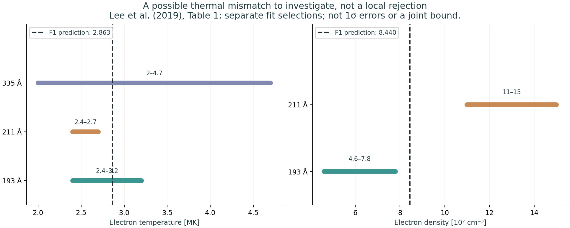
Decision: there is a possible thermal/emission mismatch worth testing, not a justified local rejection. Nor does partial range overlap confirm F1. The missing steps are spatial registration or new same-patch photometry, line-of-sight/background treatment, a valid joint emission model and the relation between electron temperature and total plasma pressure. No new thermal fit was performed.
The author-institution abstract of Downs et al. (2012) describes a thermodynamic MHD simulation of this event and distinguishes an outer fast-wave component from evolving CME-related structure. This makes a CME-related inner feature a serious comparison to retain. It does not identify our exact inner crest as a slow shock or as a material boundary. Only the abstract was accessible in this review; no local simulation state or numerical bound is imported.
The normal flow immediately ahead of the inner front directly changes the inflow used in the slow test. It must be obtained independently of the shock relation being tested. A Doppler observation measures the line-of-sight component. In our image-plane normal assumption, that direction is perpendicular to the needed normal: Doppler alone cannot supply the missing component without additional geometry/flow information. Brightness tracking also remains a pattern-speed measurement unless material motion is established.
Flow alone is insufficient: magnetic strength/direction, thermal state and the jump across the inner feature remain necessary. No universally optimal measurement or required angle precision has been established.
The next feasible bounded step with the retained data is to define one interfront aperture from the saved tracks and inspect its actual multi-channel emission and background, with explicit epoch matching, before any thermal fit. The target is the gap ahead of the inner front, not the old outer-crest aperture. If cadence or line-of-sight mixing prevents a useful constraint, report that outcome. Do not tune unknown parameters to produce slow, rerun a generic robustness program or open another event automatically.
What we measured: the two image tracks and the projected local geometry, retained from R120.
What we assumed: F1 plasma between the fronts, its uniform transfer from the outer downstream state, unmeasured absolute flows, image-plane normals and the retained source/pressure assumptions.
What RMO says: this supplied state admits a checked local slow shock. R121 has not independently selected it as the solar state.
What remains ambiguous: a slow shock, another disturbance, a CME-related structure or a changing emission pattern at the inner ridge. The current audit does not close these alternatives.
What should be measured next: the same-patch intermediate plasma state. Begin with a bounded check of the available gap emission; normal flow and magnetic constraints remain separate missing information.
The independently tracked inner EUV ridge admits a regular local slow-shock completion when its upstream state is identified with the downstream state of the retained outer-fast solution F1. An event-specific evidence audit does not independently establish this intermediate state. The published standoff-derived magnetic field describes the upstream medium of the outer shock, whereas published thermal diagnostics retain spatial-transfer and emission-model limitations. Consequently, the fast-plus-slow construction demonstrates conditional compatibility rather than identification of two solar MHD modes. Same-patch intermediate-state and inner-jump constraints are required to distinguish the surviving interpretations.
R121 is complete as a finite evidence audit. It adds one primary paper, a source record, two exact-source figures and this observer view. It retains all R120 numerical results. No new FITS, speed fit, MHD solve, DEM/NEI fit, uncertainty sweep or source-aperture registration was performed. The source set is explicitly listed in R121_evidence_record.json; absence of a constraint there is not a claim that no other observation exists.
Run build_evidence.py and build_delivery.py with the retained R110/R111/R120 records, arrays and cited PDF files. The record contains source hashes and image-display settings. RMO_R121_F1_evidence.html is self-contained; the full QuickLook also retains every previous viewer and the accepted logo.
E11 · 13 JUNE 2010 · SECOND-FRONT CHECK
One saved outer-fast state supports an inner slow shock when we assume that it describes the plasma between the fronts. The data have not yet verified that assumption or identified a solar slow shock.
Method ranges are not total errors or 1σ. The two speeds describe image patterns. The slow-shock test uses velocity relative to its assumed local plasma.
Watch both image fronts in the dynamic example above — SDO/AIA 193 Å, 13 June 2010. The original R120 controls, frames and marks are retained.
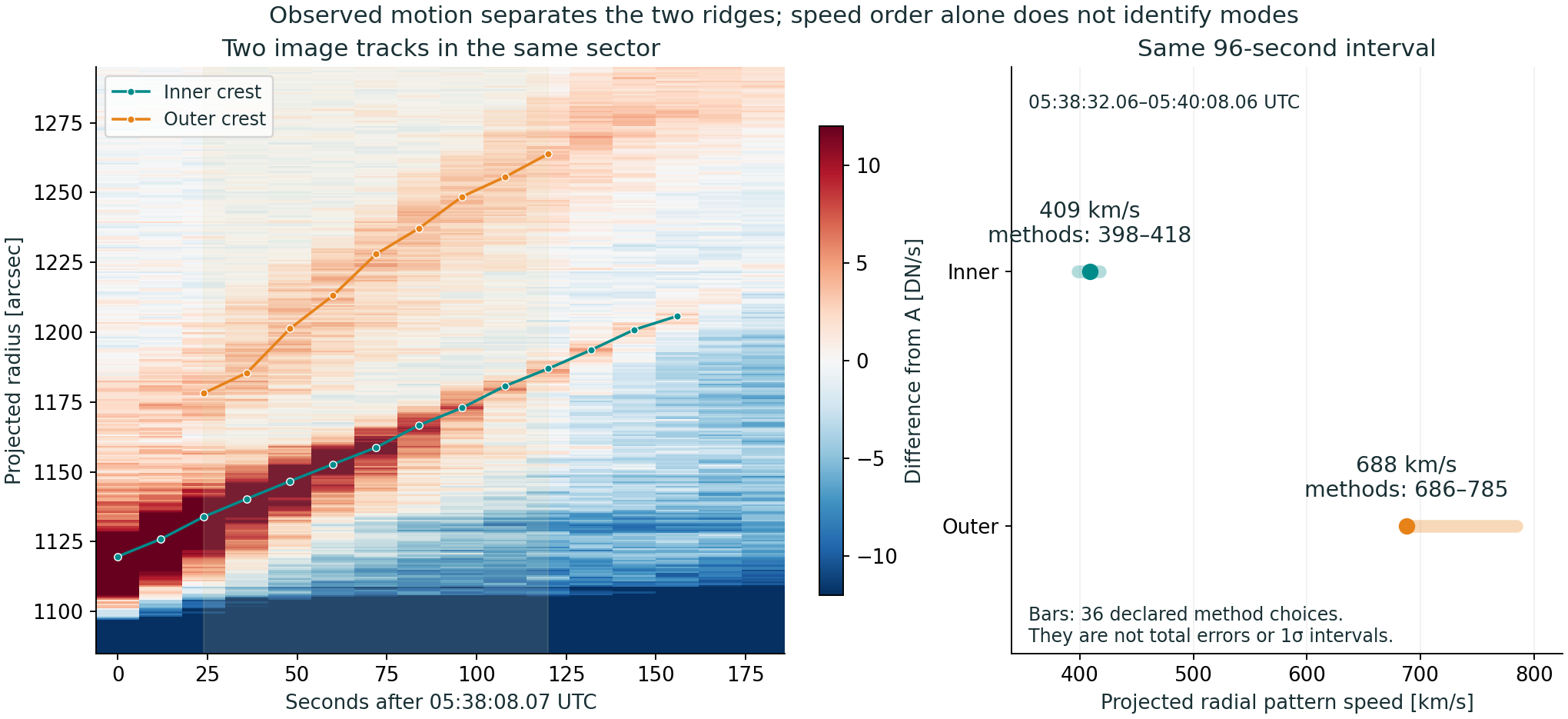
The model plasma ahead of the inner front already moves outward. The front overtakes it by about 155 km/s, although the image pattern moves at about 409 km/s. That distinction changes the wave-family test.
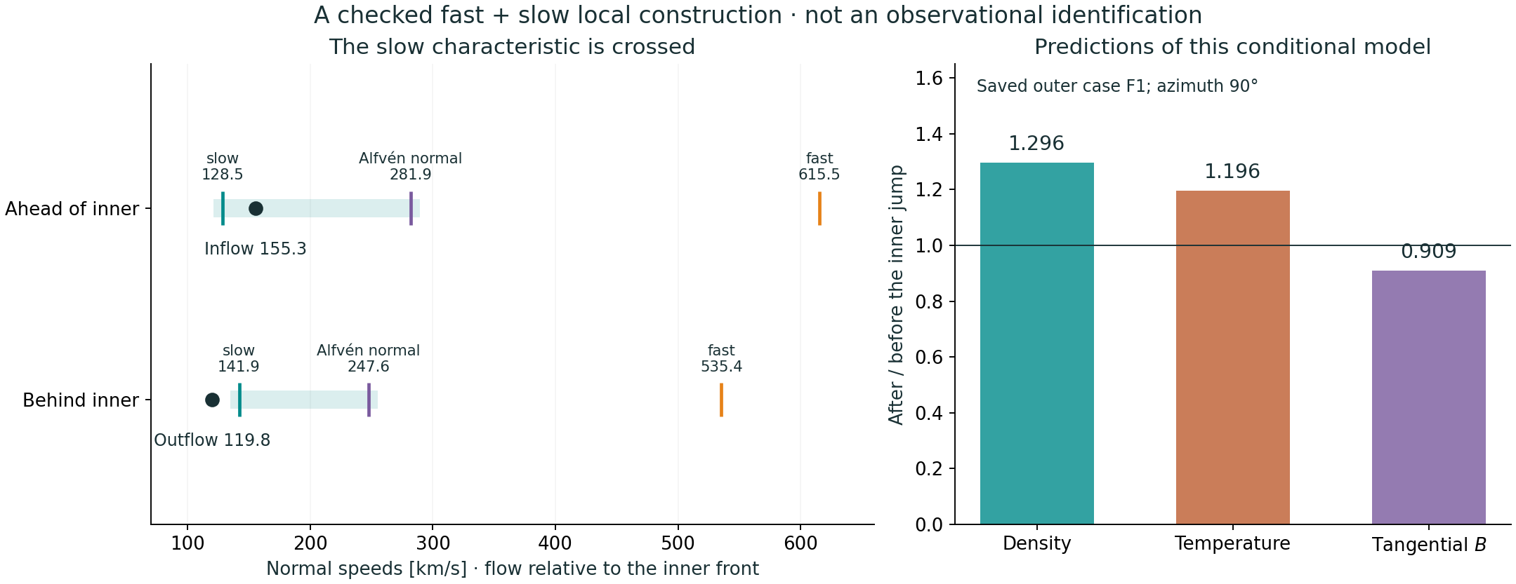
| Saved outer state | Inner slow result | What was varied |
|---|---|---|
| P | 0 / 108 completions | 36 image methods × 3 azimuths |
| F1 | 108 / 108 completions | Same fixed outer state and shared-state assumptions |
| F2 | 0 / 108 completions | 36 image methods × 3 azimuths |
This establishes compatibility under the declared conditions. It does not establish the actual intermediate plasma, a solar slow-shock discovery, or a full magnetic-explosion solution. A second fast disturbance in a different state remains an observational alternative.
| Quantity | Value / range | Origin | Source | Meaning / limitation |
|---|---|---|---|---|
| Event and feature | E11; 13 June 2010; inner 193 Å ridge, PA 116° ±1° | MEASURED / image-derived; patch is an analysis choice | 30 retained SDO/AIA FITS, R120_source_inventory.json | A projected brightness ridge. Material surface and wave family are not measured. |
| Inner motion, common interval | 409.1 km/s; method envelope 397.9–417.7 km/s | MEASURED / image-derived fit | Nine 193 Å epochs, 05:38:32.06–05:40:08.06 UTC | About 409 (−11, +9) km/s from method choices only; not total error or 1σ. |
| Inner motion, longer interval | 411.2 km/s; method envelope 407.6–419.7 km/s | MEASURED / image-derived fit | Fourteen epochs, 05:38:08.07–05:40:44.07 UTC | No expected speed entered the ridge selection. Last two weak candidates are excluded from this primary interval. |
| Inner projected normal | PA 117.52° at 05:40:08.06 UTC; method envelope 108.22–121.67° | DERIVED FROM EVENT DATA | Quadratic crest fit; 36 methods, R120_tracks.json | About 117.5° (−9.3°, +4.2°), method choices only. This is not the angle between field and front. |
| Inner effective normal speed | 408.97 km/s; declared method range 394.25–417.33 km/s | DERIVED + ASSUMED | Interval-mean radial motion projected on the endpoint normal | Both normals lie in the image plane. A mean speed and endpoint normal approximate one local state; no instantaneous 3D measurement. |
| Outer motion, common comparison | 687.5 km/s; method envelope 686.2–784.5 km/s | MEASURED / image-derived fit | Same nine epochs and same new estimator; retained R107 search windows | About 688 (−1, +97) km/s from methods only. Weak outer crests give the larger spread. R107 remains unchanged. |
| Outer-state model normalization | Vn = 705.535 km/s; outer compression 1.5625; upstream T = 1.8 MK | RETAINED MODEL + SOURCE-DERIVED + ASSUMED | R109/R110; radio and regional-temperature transfer | This model uses the original R110 normalization, not the new 687.5 km/s comparison. The difference is explicit; no hidden refit. |
| Plasma between fronts | UNKNOWN observationally; test P, F1 and F2 downstream states | ASSUMED / conditional shared-state hypothesis | All three saved regular-fast R110 points | Assume one uniform intervening state, unchanged by expansion, cooling, mixing or another wave. Same-patch transfer is not verified. |
| Absolute plasma flow | UNKNOWN; outer-upstream velocity set to zero in all components | ASSUMED | FLOW0 plus a new absolute tangential-zero assumption | R110 tangential zero was a frame choice. Here assigning it in the laboratory frame is an additional physical assumption. |
| Magnetic field and orientation | UNKNOWN as measurements; F1 intermediate model has |B| = 2.370 G | MODEL OUTPUT used in a conditional test | Unchanged R110 F1 state; field/flow azimuth examples 0°, 90°, 180° | No field value was optimized to obtain slow. Only three earlier regular-fast states were tested, not the full inverse family. |
| Inner density jump and temperature jump | UNKNOWN as observations; reference slow model predicts X = 1.296 and T ratio = 1.196 | MODEL OUTPUT, not independent input | R120 local conservation-law solution | Do not transfer the outer radio compression to the inner jump or derive density from the displayed EUV brightness. |
| Inner thermal/emission identity | 171/193/211 structures differ; one plasma component unresolved | EVENT DATA + UNKNOWN physical decomposition | Actual sparse 171/211 times; R120 marker check; R117–R118 retained | Broad 211 peaks differ from the 193 crest. The late 171 local maximum is still below its early reference. No DEM/NEI inversion. |
The wider region was sampled because the old outer-front aperture cropped the inner ridge at early times. All 30 used original FITS match their saved hashes. We used retained R113 pointing corrections, exposure normalization and bilinear sampling of unsmoothed native data. No new download, temporal interpolation, empirical residual registration, PSF correction or full level-1.5 reprocessing was performed.
Inner search windows were selected from the continuous image ridge and profiles before speed fitting, without a target speed or MHD label. Fourteen consecutive 193 Å epochs define the primary 156-second track. The two final low-contrast samples are retained as candidates only. An original-intensity leading-gradient marker gives 406.6 km/s over the same 14 epochs, with no search-boundary hit. It is a different, crest-anchored marker, not independent statistical evidence.
There are 36 declared combinations: two early references A/B, difference or log2 ratio, radial smoothing sigma 0.9/1.8/3.0 arcsec, and PA half-width 0.5/1/2 degrees. The angular smoothing sigma is 0.2 degrees. Nonpositive ratio inputs remain invalid. Every selected detector sample is finite.
All 36 matched inner fits have no boundary peak; four longer-interval methods each have one boundary hit. Six of the 36 matched outer methods each have one boundary hit; none was silently discarded. The outer comparison was repeated for one concrete reason: both speeds must use the same interval, pointing and measurement operator. It does not overwrite the older R107 track or R110 model normalization.
About 409 (−11, +9) km/s and 117.5° (−9.3°, +4.2°) are readable forms of the inner method envelopes. They are not measurement confidence intervals, hard bounds on all errors or 1σ. Projection, source association, residual image registration and plasma-state uncertainty are not included.
We tested all three previously retained regular-fast model points P, F1 and F2. No magnetic field was fitted to obtain a preferred second mode. Each saved outer-downstream state was, in turn, assumed to be the uniform state immediately ahead of the inner front. Expansion, mixing, cooling, conduction and intervening waves were neglected. This spatial and temporal transfer is unverified.
Both front normals were assumed to lie in the image plane. The inner endpoint normal and its 96-second mean speed give an effective normal pattern speed of 408.968 km/s. The old outer model keeps Vn = 705.535 km/s. The original R110 radio-to-patch association, regional temperature, pure fully ionized hydrogen, Te = Tp and gamma = 5/3 remain conditional.
The laboratory velocity ahead of the outer shock was set to zero in all components. The tangential part is a new physical assumption: a zero tangential velocity in R110 alone was a frame choice. Unknown tangential field/flow orientation around the outer normal was tested at azimuths 0°, 90° and 180°. These azimuths are not measured field angles.
For each resulting inner upstream state, the full local ideal-MHD jump relations were reduced to an energy polynomial in compression. The trivial no-jump root was removed; all remaining real compressive roots in the stated ideal-gas range were enumerated. Positive pressure, entropy production, flux conservation and characteristic ordering were checked. The unchanged RMO diagnostic received the states and front speed, without a requested type label.
The exact_synthetic flag inside each solver request means that the constructed model point is evaluated deterministically. It does not describe the uncertainty or origin of the solar inputs.
| Quantity | Ahead of inner front | Behind inner front |
|---|---|---|
| Normal plasma speed relative to front [km/s] | 155.269 | 119.763 |
| Slow characteristic speed [km/s] | 128.534 | 141.929 |
| Normal Alfvén speed [km/s] | 281.888 | 247.568 |
| Fast characteristic speed [km/s] | 615.515 | 535.384 |
| Density, normalized to inner upstream | 1 | 1.296476 |
| Common Te = Tp [MK], model only | 2.862823 | 3.423906 |
| Tangential field, normalized to inner upstream | 1 | 0.909421 |
Ahead of the inner jump, the relative inflow lies above the slow speed and below the normal Alfvén speed: 128.5 < 155.3 < 281.9 km/s. Behind it, the outflow is below the new slow speed: 119.8 < 141.9 km/s. Density and entropy increase, while tangential magnetic field decreases. This is a regular slow-shock crossing; simply moving more slowly than the outer front would not establish it.
All central slow solutions pass the separately evaluated mass, normal/tangential momentum, induction and energy flux relations; their maximum scaled residual is 4.25 × 10⁻¹⁶. A separate scalar energy-root calculation agrees with the polynomial root. The unchanged RMO diagnostic returns SUPPORTED_LOCAL_CLASS / slow_shock. Restoring a common laboratory-normal velocity boost leaves the diagnosis unchanged.
F1 gives inner compression 1.232, 1.296 and 1.369 at the three central azimuths. For P and F2, no regular slow completion is found under the same closure. Analytic azimuth bounds at the central geometry prove that the upstream slow condition holds for F1 and fails for P/F2 over all azimuths. The full finite-amplitude jumps themselves were solved only at the three stated azimuths.
First define the plasma just ahead of the inner front. In this hypothesis it is already behind the outer fast shock. Its density, pressure, field and velocity therefore differ from the undisturbed corona. Copying the outer upstream state to both fronts would be a different physical model.
The reference F1 intermediate state has density 1.412 × 10⁻¹³ kg/m³, common Te = Tp = 2.863 MK and total field 2.370 G. Its field makes an acute angle of 59.94° to the inner normal after the stated geometric transformation. These are conditional model values. The measured projected normal PA 117.52°, the field angle and the free azimuth 90° are three different angles.
Use the relative normal inflow w₁ = Vn − u₁n. Let a² = gamma p/rho, vA² = B²/(mu0 rho), and cAn² = Bn²/(mu0 rho). The local fast and slow speeds obey c²_fast,slow = [(a² + vA²) ± sqrt((a² + vA²)² − 4 a² cAn²)] / 2. They are calculated separately in each state; an image pattern speed is not a substitute.
For the regular non-degenerate slow shock tested here, the upstream order must be cslow,1 < w₁ < cAn,1. Downstream, 0 < w₂ < cslow,2. Together with positive density/pressure, increased entropy and all conservation relations, this is the local admissibility check. A slow-looking feature or a low image speed alone satisfies none of those tests.
At this fixed F1 upstream state and Vn = 408.968 km/s, the upstream ordering alone requires approximately 127.1 < u₁n < 280.4 km/s. The assumed intermediate normal flow 253.7 km/s falls inside. This interval is only a necessary upstream speed condition at fixed field, pressure and geometry; it is not an observational flow interval, a full existence proof over the interval, or a tolerance on the solution.
We then solve the downstream state rather than assuming the second inequality. The solution gives w₂ = 119.763 km/s < cslow,2 = 141.929 km/s, density ratio 1.296, field-tangent ratio 0.909 and positive entropy production. This is the point where the conditional hypothesis becomes a checked slow-shock solution.
The other saved intermediate states explain why two fronts do not uniquely select two modes. P has too small a normal Alfvén speed for the inner inflow to be a regular slow shock. F2 has a slow speed higher than that inflow. F1 lies between the appropriate characteristics. Their common outer compression does not fix the inner wave family.
This local construction gives no prediction of the global blast shape, source energy, piston history, total wave fan or source-to-front timing. Those would have to follow from a specified initial/boundary-value problem. Agreement with a remembered fast/slow magnetic explosion cannot replace that comparison.
| Saved outer state | Slow completions | Predicted inner compression range | Scope |
|---|---|---|---|
| P | 0 / 108 | — | 36 coupled inner-track methods × 3 azimuths |
| F1 | 108 / 108 | 1.0068–1.6442 | Same fixed outer model and shared-state closure |
| F2 | 0 / 108 | — | Same fixed outer model and shared-state closure |
The F1 slow completion survives every declared coupled marker/normal method and the three chosen azimuths. The 108/108 count is not a probability, a confidence level or proof over a continuous physical uncertainty domain. Some completions approach the weak-jump limit. The compression range describes model outputs, not measured solar compression.
The earlier outer radio/temperature sweep was not repeated or transferred to the new inner state. The full R110 inverse family, out-of-plane normals, unknown absolute flows, state evolution between fronts and a full azimuth continuum of finite jumps are not certified by this test. Thus the slow result is stable to these particular image-method choices, while remaining conditional on the much stronger plasma-state assumptions.
The four actual 171 and 211 science epochs contain inner-neighborhood candidate peaks with approximate fitted pattern rates of 403 and 402 km/s. Their maxima are not forced to coincide with the 193 ridge. The 211 enhancement is broad; at the late 171 epoch the local maximum is still 1.25 DN/s below reference A. Calling it a positive bright front would be wrong.
The sparse asynchronous exposures do not measure a precise inter-channel lag or isolate one plasma component. No temperature fit, density jump, radiometric significance or wave family follows from these displayed colors. The retained R117 native-aperture measurements and the R111 temperature-transfer restriction are unchanged.
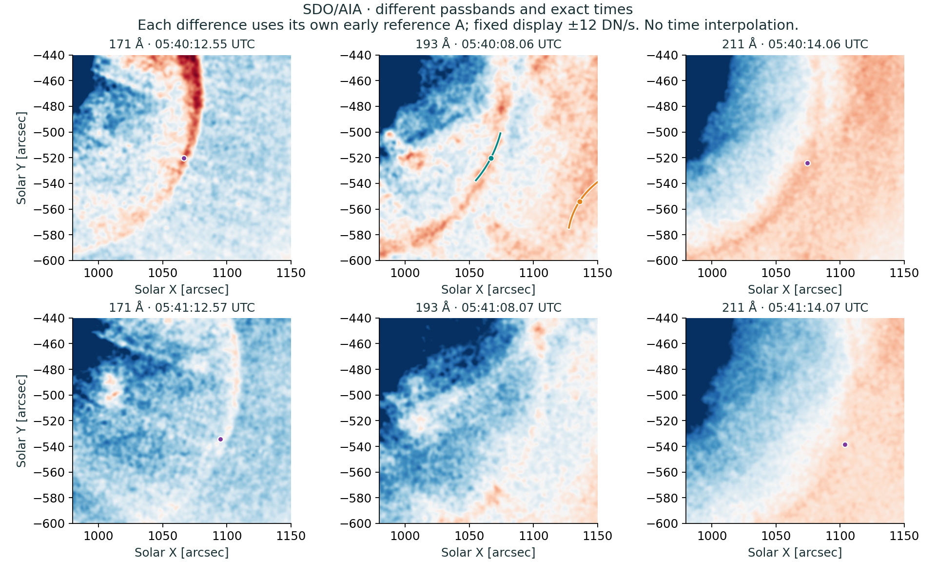
| Question | Result | Limit |
|---|---|---|
| Two separate image tracks | Supported in the selected interval and sector | Inner about 409 km/s; outer about 688 km/s. This is image motion, not a mode assignment. |
| A conditional fast + slow construction | Established for saved outer-fast F1 and the explicit uniform-state hypothesis | A complete local inner slow jump satisfies conservation, entropy and characteristic ordering. |
| The same slow construction for P or F2 | Not supported in the tested closure | Their inner upstream states fail the necessary slow-shock speed ordering at the central geometry. |
| A second regular fast shock | Not supported by the tested central P/F1/F2 shared states | In those states the inner relative inflow is below the fast speed. Different actual intervening plasma can change this result. |
| A solar slow-shock discovery | Not established | The observations have not selected F1 or measured the required intervening and inner-downstream states. |
| CME boundary, changing emission or another disturbance | Still observational alternatives | Morphology and two speed tracks alone do not settle them. No material-surface identification is imposed. |
| A Korobeinikov magnetic-blast solution | Not verified | Exact remembered source remains unresolved; this is a local two-jump construction, not a global blast solution or full Riemann fan. |
A useful next independent quantity is the normal velocity of the plasma between the two fronts at the selected patch. It changes the inner inflow through w = Vn − u_between,n. In the reference conditional slow case, the intermediate projected normal flow is about 254 km/s, leaving only about 155 km/s relative inflow despite the roughly 409 km/s image speed.
Flow alone will not identify the mode. It must be combined with same-patch magnetic direction/strength and thermal constraints, and ultimately compression across the inner feature. Measuring a compressive transition with decreasing tangential field would directly test the slow hypothesis; a different state can restore a different interpretation. No globally optimal measurement or required angular precision has been established here.
What we measured: an inner image trajectory and projected normal, a matched outer trajectory, and actual multi-channel image structure.
What we assumed: a uniform intermediate state copied from one saved outer solution, laboratory upstream flow zero including its tangential part, image-plane normals, source transfers and ideal-MHD pressure closure.
What RMO says: F1 supports a fully checked local inner slow shock; the other two saved regular-fast points do not support that slow completion in the same closure.
What remains ambiguous: whether the solar inner ridge is that slow shock, another disturbance, a CME-related boundary or an emission pattern; the intermediate plasma has not been independently determined.
What should be measured next: the same-patch intermediate plasma velocity/state, then compare its predicted inner jump with independent compression/field constraints. No new event or generic robustness program starts automatically.
Ma et al. (2011), Ma et al. (2011), discuss this event as an outer EUV dome ahead of a CME bubble. That interpretation is source context, not our independent proof of a material boundary or two colliding CMEs. Published source speeds were not used as target values for the new inner track.
The oblique ideal-MHD jump framework is described by R. Fitzpatrick, Oblique MHD shocks. The numerical states, independent checks and method comparisons above are new R120 calculations.
The exact Korobeinikov magnetic-explosion reference remembered in discussion has not been established. A local fast + slow construction does not verify an author-specific global explosion solution. No such historical or global-model claim is made.
Reproduce with sample_inner.py, track_inner.py, check_markers.py, check_shared_state.py, check_joint_sensitivity.py, build_figures.py and build_result.py. sample_inner.py requires Astropy and the retained pointing table. Full input paths and hashes are in R120_source_inventory.json. Solver source and the unchanged R110 input record are included in the checkpoint. No original FITS bytes were changed.
R120 is complete for this bounded question. The R119 outer-front result and all earlier event viewers are retained. The next decision concerns independent plasma constraints, not an automatic new solver sweep.
E11 · 13 June 2010 · result with current constraints
The event now has a complete bounded result: measured image motion and channel histories, explicit source-transferred inputs, checked central model states, and a conditional exclusion with a quantified missing-flow requirement. A complete measured pair of plasma states is still unavailable.
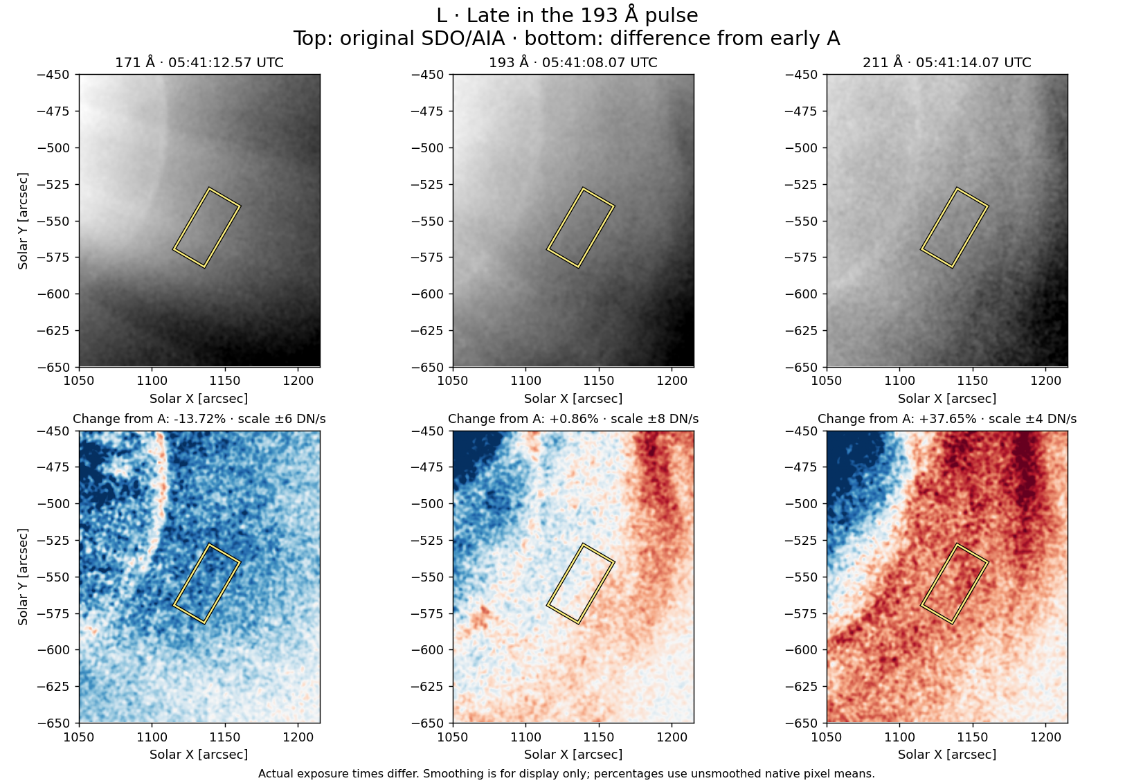
| Question | Result | Scope |
|---|---|---|
| Outer-front image motion | Established within the selected marker, sector and fit interval. | Measured pattern, with geometric/plasma-frame interpretation still conditional. |
| A fast local jump | Compatible: the saved R110 P,F1,F2 states pass conservation, entropy and characteristic checks. | Central C0 inputs/closure; no unique field or solar identification. |
| A regular slow local jump at C0 | Excluded; now the exclusion also holds throughout the declared radio/T box at fixed G0 speed and zero flow. | One planar ideal-MHD jump only; source transfer, geometry and flow assumptions remain. |
| Switch-on / field-reversing completions | Saved degenerate or admissibility-unresolved R110 examples remain. | They are not promoted to physical solar solutions or silently removed. |
| Two MHD modes in the images | Not established. | Two image structures or differing channels are insufficient for a fast+slow assignment. |
| Unique solar wave family / magnetic field | Unresolved with the current independent observations. | Conditional compatibility is the final result of this bounded event analysis. |
| Quantity | Value / range | Origin | Source | Uncertainty or assumption |
|---|---|---|---|---|
| Event/patch | 2010-06-13; PA 116 outer 193 crest; fixed 24″×48″ region | MEASURED image-derived selection; ANALYSIS CHOICE | R106–R107/R112; original AIA | A sky patch, not a fluid parcel or a measured isolated LoS component. |
| Radial pattern speed | 707.5 km/s over 05:38:32.06–05:40:08.06 | MEASURED image-derived fit | R107 retained result | 687–718km/s estimator spread, not 1σ or full bounds;60-s mean576.7km/s remains separate. |
| Normal and inflow | Image normal PA120.28°; G0 Vn705.5km/s; reference u1n=0 | DERIVED + ASSUMED | R106/R109/R110 | 113–126° estimator spread is not full uncertainty. LOS tilt, actual flow and time-dependent 3D speed are unknown. |
| Channel histories | Late 171−13.72 to−13.76%;193+0.86 to+0.96%;211+37.65 to+38.09% | DERIVED FROM EVENT DATA | R117; unsmoothed native means | Two early-reference choices; not total error or sigma. Actual group times span up to 6.01s. |
| Radio lanes | 132±5 /165±15MHz; joint bounds 127–137 /150–180 | SOURCE-DERIVED + ASSUMED event-patch transfer | Ma2011; retained R108/R109 | Second harmonic and upstream/downstream split interpretation; source localization to this patch unproved. Bounds are scenario choices, not certified confidence intervals. |
| Density/compression | ne1=5.40×10^7cm^-3; X=1.5625; X bounds1.199–2.009 | DERIVED + ASSUMED transfer | Same radio pair | ne1, ne2 and X share the frequencies; they are not independent evidence. |
| Upstream temperature/pressure | T=1.8±0.4MK; p=2ne kB T; rho=mp ne | SOURCE-DERIVED regional T + ASSUMED closure | R108/R109, Ma/Kozarev | Pure fully ionized H; Te=Tp; gamma5/3. Patch transfer and composition/equilibration uncertainties are not covered by±0.4MK. |
| Magnetic field and direction | No independent B or theta_Bn bound | UNKNOWN input; conditional model output | R110 retained inverse family | Three checked ordinary fast examples give B1=1.474,1.597,1.753G, not a measured field range. |
| Downstream thermodynamics / one emitting component | Not independently determined for this patch | UNKNOWN | R111 and new R117–R118 evidence | Do not import Lee2019 projected temperature-fit range as a hard patch constraint or equate DEM electron T to common Te=Tp. |
| Upstream normal plasma flow | No measured bound | UNKNOWN; u1n=0 only reference | No matched local plasma-flow diagnosis in retained input set | R119 derives a conditional requirement on this quantity; it does not measure it. |
| Saved case | B₁ [G] | Angle [°] | Equivalent T₂ [MK] | Saved status |
|---|---|---|---|---|
| R110_P | 1.474 | 90.00 | 2.752 | SUPPORTED_LOCAL_CLASS |
| R110_F1 | 1.597 | 41.89 | 2.863 | SUPPORTED_LOCAL_CLASS |
| R110_F2 | 1.753 | 16.49 | 3.127 | SUPPORTED_LOCAL_CLASS |
| R110_S | 1.902 | 0.00 | 3.535 | DEGENERATE_NOT_CLASSIFIED |
| R110_I1 | 2.176 | 18.88 | 4.573 | OTHER_OR_UNRESOLVED |
| R110_I2 | 2.534 | 32.96 | 6.273 | OTHER_OR_UNRESOLVED |
These results come unchanged from R110. They are examples at the central inputs, not error bars or bounds on B. Degenerate and admissibility-unresolved states remain explicit. No earlier solver check is rerun.
The retained scenario bounds are 132±5MHz,165±15MHz and1.8±0.4MK. They imply compression1.199–2.009. Frequency-derived density,pressure and compression remain linked; the inputs are not independently shuffled. These are hard scenario bounds, not 1σ and not certified source-transfer errors.
For one ideal-MHD jump, pure H with Te=Tp and gamma5/3, at the fixed G0 effective speed and u₁ₙ=0, the regular-slow exclusion holds throughout this whole box. It is established by the sign of the transition equation, not by checking only a grid of examples.
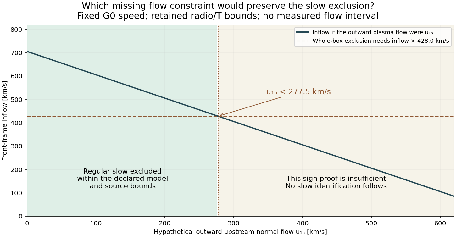
At exact central radio/T inputs only, the corresponding flow limit is 396.9km/s. Beyond either relevant limit, this proof becomes insufficient; slow is not thereby identified and fast is not automatically excluded. Unknown3D geometry, source matching and pressure closure remain outside this bound.
With r=ρ₂/ρ₁, b=p₁/(ρ₁w₁²), h=Bₙ²/(μ₀ρ₁w₁²), use N=4−r−5br and S=r+5−2rh(4−r). The retained RH relation requires Bₜ₁²=2N(1−rh)²/(rS) in normalized units.
Regular slow requires h>1. Here1<r<2.5, so S(1)=(r−1)(2r−5)<0 and S decreases with h. At zero flow N≥1.25836 across the box; Bₜ₁² would be negative. The purely parallel gas-jump exception instead needs r≥2.93080, outside the radio range. These treat the zero-field-tangent exception separately.
The sufficient inflow bound is w₁>max sqrt[5(p₁/ρ₁)r/(4−r)]=428.0218km/s. With Vₙ=705.5353km/s and w₁=Vₙ−u₁ₙ this gives u₁ₙ<277.5136km/s. No full Riemann fan, intermediate-shock admissibility or fast-family existence over the whole uncertainty box is certified.
| Second feature: what is available? | Current status |
|---|---|
| Visible inner structure | Present in some profiles; a candidate feature, not yet a separately tracked wave. |
| Its own normal and speed | Not independently reconstructed. First establish a continuous ridge across images and its own time interval. |
| Its own plasma constraints | No matched density/compression, flow or magnetic constraints assigned to this inner feature. Outer-front radio inputs cannot be copied. |
| MHD-mode result | UNKNOWN. A second wave, a CME-related boundary or evolving emission remain alternatives. |
| Scope of the slow exclusion | Applies only to the outer-front local jump and its declared inputs. It does not exclude a slow component at another front. |
The inner feature can be tested with RMO in principle, but it needs its own observational record. The first missing step is an independent track and normal, before assigning plasma states or a mode. Being slower in an image would not by itself make it a slow MHD wave.
| Explanation | Evidence | Still needed |
|---|---|---|
| A moving outer disturbance with thermal/emission evolution behind it | Consistent with the distinct channel histories and broader 171/211 changes. | No unique T, ionization or density history fitted. |
| Outer front plus an inner CME-related feature | An inner image feature and a separated outer 193 ridge are visible in some phases; Ma et al. describe a dome ahead of a CME bubble. | Inner-feature identity/trajectory and local plasma state are not independently reconstructed here. |
| Two distinct MHD wave families, such as fast and slow | Possible hypothesis; different channel intensities do not establish it. | Need two separable trajectories/states and characteristic-speed tests for each. R110 describes one local jump only. |
| Line-of-sight/background mixtures and response effects | Not separated by a fixed image-plane aperture or three channels alone. | No unique component separation, residual-registration budget or joint emission fit. |
The current data do not determine a second pair of states and its characteristic crossing. A slow component elsewhere in a multiwave structure is not excluded by a bound on the one local jump used in C0.
This is the shared index, not a claim that all 12 records have been reconstructed. E11 has the new bounded outcome. Other saved studies/controls retain their earlier scope.
| Card | Date | Title | Diagnostics / provenance | Result at this checkpoint | Next question |
|---|---|---|---|---|---|
| E01 | 2007-05-19 | One event, different measured speeds | Original catalogue constraints retained; protocol audit not updated here | Retained catalogue/study card; no new event-level assessment in this block | Choose one bounded question when this card is opened |
| E02 | 2010-07-27 | Two distinct propagating structures | Original catalogue constraints retained; protocol audit not updated here | Retained catalogue/study card; no new event-level assessment in this block | Choose one bounded question when this card is opened |
| E03 | Not fixed in the current card | Wave trains ahead of CME restructuring | Original catalogue constraints retained; protocol audit not updated here | Retained catalogue/study card; no new event-level assessment in this block | Choose one bounded question when this card is opened |
| E04 | 2011-02-15 | Weak compression with a thermal response | Original catalogue constraints retained; protocol audit not updated here | Retained catalogue/study card; no new event-level assessment in this block | Choose one bounded question when this card is opened |
| E05 | 2011-02-16 | Fast image motion, modest Doppler response | Original catalogue constraints retained; protocol audit not updated here | Retained catalogue/study card; no new event-level assessment in this block | Choose one bounded question when this card is opened |
| E06 | 2011-06-07 | CASHeW: front, peak and back | Original catalogue constraints retained; protocol audit not updated here | Retained catalogue/study card; no new event-level assessment in this block | Choose one bounded question when this card is opened |
| E07 | 2013-12-12 | CASHeW: a C-class front | Original catalogue constraints retained; protocol audit not updated here | Retained catalogue/study card; no new event-level assessment in this block | Choose one bounded question when this card is opened |
| E08 | 1998-06-13 | Harra control: front is not filament | See retained control evidence and limits | Saved control retained; no reopened audit | No new control work in this block |
| E09 | 2015-06-22 | IRIS slow-shock literature comparison | Original catalogue constraints retained; protocol audit not updated here | Retained catalogue/study card; no new event-level assessment in this block | Choose one bounded question when this card is opened |
| E10 | 2011-01-27 | Vršnak co-authored catalogue: a B-class example | Original catalogue constraints retained; protocol audit not updated here | Retained catalogue/study card; no new event-level assessment in this block | Choose one bounded question when this card is opened |
| E11 | 2010-06-13 | An EUV dome ahead of a CME bubble | Image geometry/motion and channel histories measured; radio/T transferred conditionally; flow/B unknown | R119 bounded result: conditional fast compatibility; regular-slow exclusion within declared bounds; solar family unresolved | Same-patch plasma association; quantified conditional flow requirement |
| G2009 (separate) | 2009-02-13 | Worked stereoscopic geometry example; T. Podladchikova et al. (2019) | Worked stereoscopic geometry case | Saved geometry comparison retained; no complete MHD inversion asserted | Keep its original scope |
Ma et al.(2011) describe the outer dome and associated CME bubble and provide the radio diagnostics used conditionally. Lee et al.(2019) model nonequilibrium-ionization responses; the saved R111 audit limits transfer of their temperatures to our patch.
We cannot yet rank one globally optimal new measurement or prescribe an accuracy on the field angle. We can identify the unverified source-to-patch association and quantify one useful normal-flow requirement. This closes the present E11 block with its actual information content. No new event, download or physical fit is automatically launched.
E11 · 13 June 2010 · no new data
The profiles distinguish the outer 193 ridge from broader changes and an inner feature. They do not establish two independently classified waves. A front, a CME-related rim and an emission region can be separate image features with different physical roles.
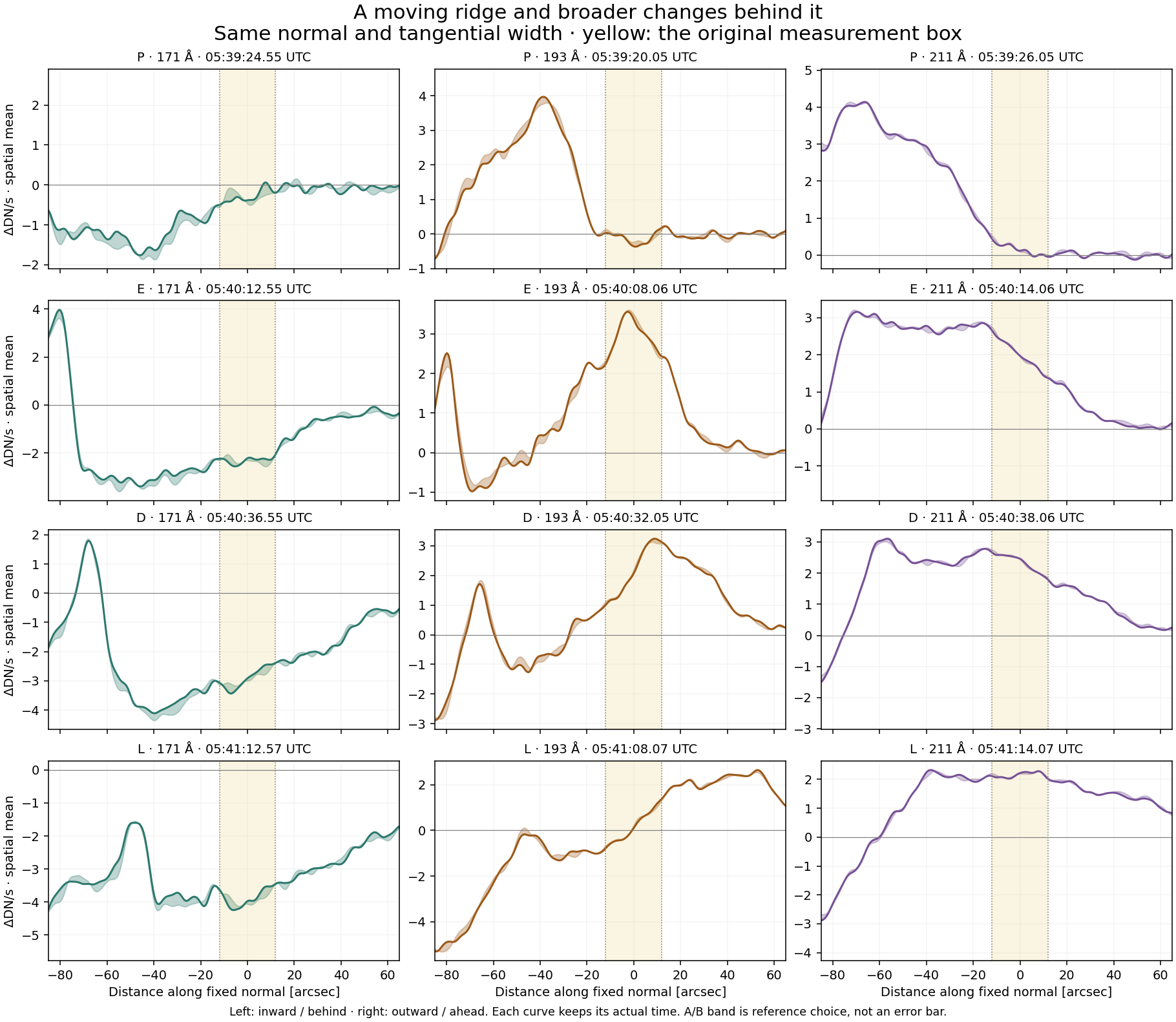
| Explanation | What the current data show | Limit |
|---|---|---|
| A moving outer disturbance with thermal/emission evolution behind it | Consistent with the distinct channel histories and broader 171/211 changes. | No unique T, ionization or density history fitted. |
| Outer front plus an inner CME-related feature | An inner image feature and a separated outer 193 ridge are visible in some phases; Ma et al. describe a dome ahead of a CME bubble. | Inner-feature identity/trajectory and local plasma state are not independently reconstructed here. |
| Two distinct MHD wave families, such as fast and slow | Possible hypothesis; different channel intensities do not establish it. | Need two separable trajectories/states and characteristic-speed tests for each. R110 describes one local jump only. |
| Line-of-sight/background mixtures and response effects | Not separated by a fixed image-plane aperture or three channels alone. | No unique component separation, residual-registration budget or joint emission fit. |
Conclusion: the same projected aperture does not isolate one common thermodynamic component. Do not identify fast/slow from which channel is bright, or equate two profile maxima with two characteristic families.
Only saved R117 arrays are used. Bilinear profile sampling,80 tangential positions spaced 0.6″; display Gaussian sigma 1.8″. Fixed inward/aperture/outward windows are analysis choices. No new track, speed, lag or plasma inversion.
Ma et al.(2011) describe a dome ahead of a CME bubble in this event. That source interpretation is not a new identification of modes in our patch.
13 June 2010 · E11 · original SDO/AIA
The channels do not return toward their early values together. Near 05:41:10 UTC, 171 Å is 13.72–13.76% dimmer, 193 Å remains only 0.86–0.96% brighter, and 211 Å remains 37.65–38.09% brighter than the selected early references.
Same place does not automatically mean one isolated plasma component. The images show a narrower moving bright band in193 Å alongside broader changes in171 and 211 Å. These are measured passband histories. Temperature, density, emitting depth and overlapping structures are not yet separated.
Top row: originals. Bottom row: each channel minus its own early A image. Yellow marks the unchanged measurement box. Start with P, then E, D and L. A/B are also available on the slider.

Original images: SDO/AIA. Each panel prints its actual UTC exposure time. Play advances one selected phase per second; this is a sparse comparison, not a uniform-cadence movie. No intermediate images are generated.
| Phase | 171 Å · A / B | 193 Å · A / B | 211 Å · A / B |
|---|---|---|---|
| P | -0.99% / -1.03% | -0.60% / -0.50% | +2.46% / +2.78% |
| E | -8.16% / -8.20% | +13.08% / +13.20% | +34.82% / +35.24% |
| D | -10.24% / -10.28% | +9.55% / +9.66% | +40.88% / +41.32% |
| L | -13.72% / -13.76% | +0.86% / +0.96% | +37.65% / +38.09% |
P: near the last low 193 sample before its rise. E: near the sampled 193 maximum. D: during its decline. L: near its last low excess. A / B lists two reference choices, not two measurements of the event or a statistical error.
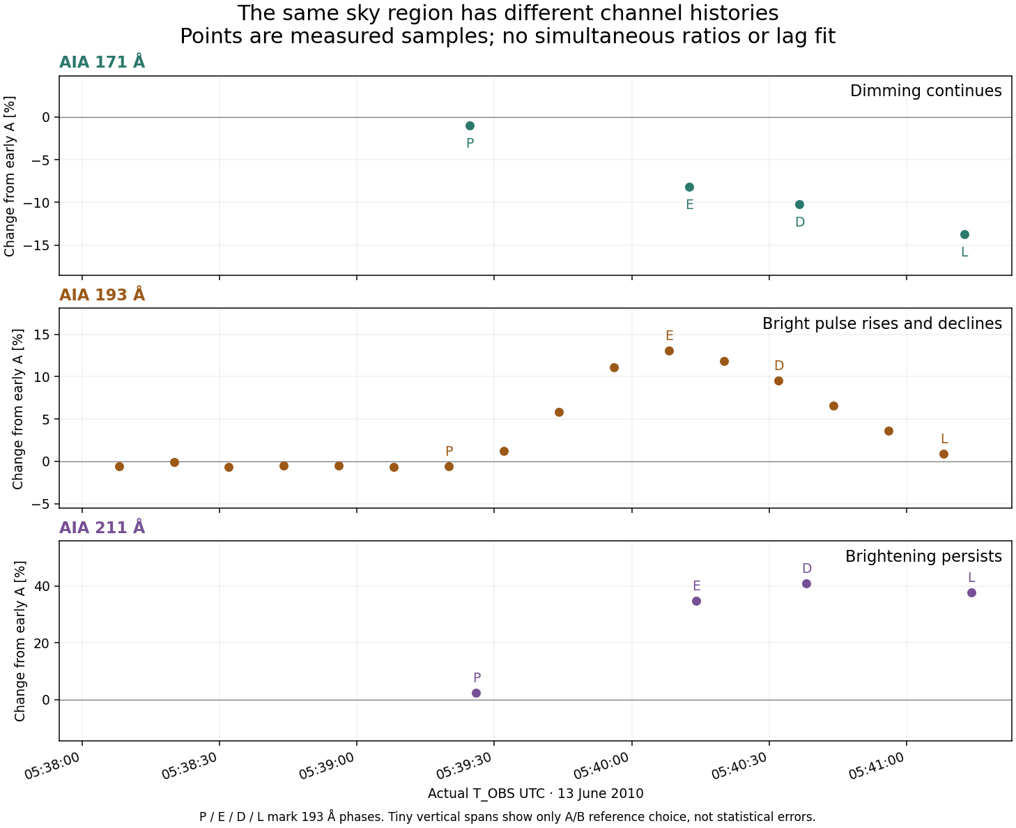
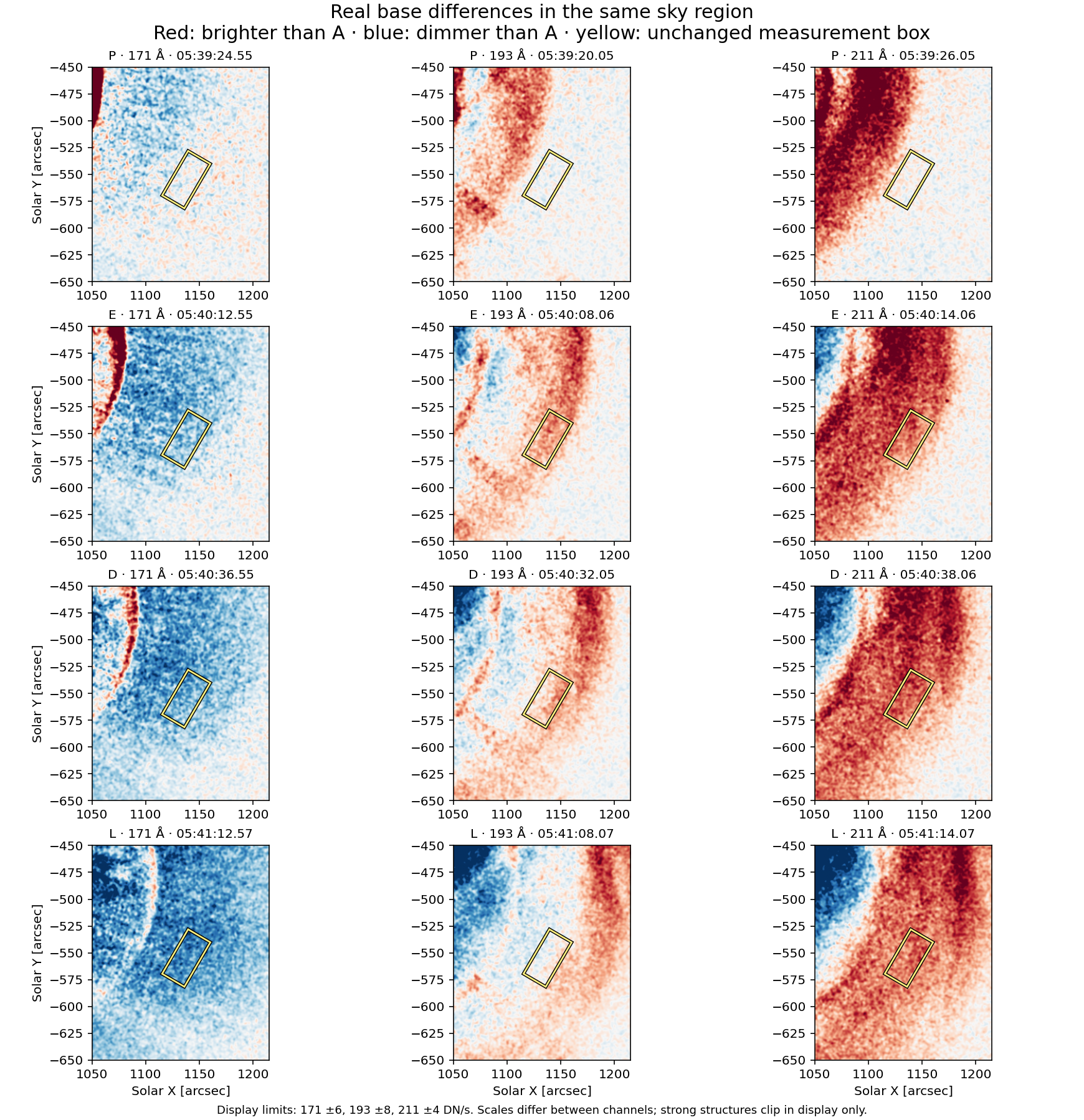
Image brightness and difference scales are fixed across times within each channel, but differ between channels. Red/blue strength cannot be compared as calibrated photon flux. Strong inner structures clip in the display; quantitative native means are unclipped.
A single bright193 image cannot supply the time history of the other channels. Even when193 has declined close to its early level,171 and 211 retain changes with opposite signs. The observed region has channel-dependent evolution.
This is a reason to examine spatial components and the response to plasma conditions before converting brightness into compression. It is not a unique proof of heating, cooling, evacuation or any wave family. No DEM, density or magnetic inference is performed here. Earlier conditional R110 solutions are neither selected nor rejected, and the R111 restriction on importing an unmatched published temperature remains.
The 211 sample at 05:40:38.06 is higher than its sample at 05:40:14.06 and its final sample at 05:41:14.07. This is a largest saved211 sample, not an accurately timed physical peak or a measured lag relative to193.
For each value, A/B changes only the selected early reference. This is not 1σ, not a total error bar and not a bound on all possible backgrounds. Earlier reference fluctuations, residual registration, noise, scattered light and background evolution are not fully separated.
171 exposures are about 4.49–4.52s later than their grouped193 exposures;211 is about 5.96–6.01s later. The time offsets are known metadata, not uncertainty estimates. At late L, the final193 exposure precedes171/211; there is no later 193 frame here to make the group simultaneous. No cross-channel ratio or temporal interpolation is used.
| Input | Source | Origin | Meaning / limit |
|---|---|---|---|
| Six new event images | Original SDO/AIA level-1 FITS, VSO/NSO delivery | MEASURED detector samples | 171 and 211 at three prespecified epochs. Not direct temperature or density measurements. |
| Earlier A/B/E samples and193 history | R114 and R116 records and image arrays | DERIVED FROM EVENT DATA · retained | Means are reused exactly. No repeated R107 tracking or speed fit. |
| New aperture means | This work: native pixel-centre samples divided by exposure | DERIVED FROM EVENT DATA | No smoothing or clipping in photometry. No full noise/error estimate. |
| Sky box and references | R112 polygon; R114 early A and B | ANALYSIS CHOICE | Same projected region, not necessarily the same plasma or isolated emitting component. |
| Pointing | Retained R113 event-day calibration and header transformation | SOURCE-DERIVED calibration | Common sky coordinates; residual inter-channel alignment is not quantitatively bounded. |
| Phase labels P/E/D/L | Selected using the saved193 history before new brightness inspection | ANALYSIS CHOICE | Exact times differ by4.49–6.01s from 193. Labels do not assign extrema to171/211. |
| Thermodynamic/vector plasma state | No new values assumed or fitted | UNKNOWN / unresolved | Radio association remains conditional; R111 temperature-transfer restriction stays. |
| Å | Phase | T_OBS UTC | Mean DN/s/native pixel | Change from A | Change from B | Offset from 193 [s] |
|---|---|---|---|---|---|---|
| 171 | A | 05:35:12.57 | 28.34315 | +0.00% | -0.04% | +4.50 |
| 171 | B | 05:36:12.55 | 28.35503 | +0.04% | +0.00% | +4.46 |
| 171 | P | 05:39:24.55 | 28.06348 | -0.99% | -1.03% | +4.50 |
| 171 | E | 05:40:12.55 | 26.02969 | -8.16% | -8.20% | +4.49 |
| 171 | D | 05:40:36.55 | 25.44125 | -10.24% | -10.28% | +4.50 |
| 171 | L | 05:41:12.57 | 24.45425 | -13.72% | -13.76% | +4.50 |
| 193 | A | 05:35:08.07 | 22.81437 | +0.00% | +0.10% | +0.00 |
| 193 | B | 05:36:08.09 | 22.79135 | -0.10% | +0.00% | +0.00 |
| 193 | P | 05:39:20.05 | 22.67675 | -0.60% | -0.50% | +0.00 |
| 193 | E | 05:40:08.06 | 25.79895 | +13.08% | +13.20% | +0.00 |
| 193 | D | 05:40:32.05 | 24.99212 | +9.55% | +9.66% | +0.00 |
| 193 | L | 05:41:08.07 | 23.01030 | +0.86% | +0.96% | +0.00 |
| 211 | A | 05:35:14.07 | 5.70887 | +0.00% | +0.32% | +6.00 |
| 211 | B | 05:36:14.05 | 5.69094 | -0.31% | +0.00% | +5.96 |
| 211 | P | 05:39:26.05 | 5.84914 | +2.46% | +2.78% | +6.00 |
| 211 | E | 05:40:14.06 | 7.69670 | +34.82% | +35.24% | +6.00 |
| 211 | D | 05:40:38.06 | 8.04268 | +40.88% | +41.32% | +6.01 |
| 211 | L | 05:41:14.07 | 7.85835 | +37.65% | +38.09% | +6.00 |
| Phase / Å | File identifier | Project path |
|---|---|---|
| A / 171 | aia__lev1:171:1055482547 | observational_pilot/background_R114/raw/aia__lev1_171_1055482547.fits |
| B / 171 | aia__lev1:171:1055482607 | observational_pilot/background_R114/raw/aia__lev1_171_1055482607.fits |
| P / 171 | aia__lev1:171:1055482799 | observational_pilot/multichannel_R117/raw/aia__lev1_171_1055482799.fits |
| E / 171 | aia__lev1:171:1055482847 | observational_pilot/epoch_R113/raw/aia__lev1_171_1055482847.fits |
| D / 171 | aia__lev1:171:1055482871 | observational_pilot/multichannel_R117/raw/aia__lev1_171_1055482871.fits |
| L / 171 | aia__lev1:171:1055482907 | observational_pilot/multichannel_R117/raw/aia__lev1_171_1055482907.fits |
| A / 193 | aia__lev1:193:1055482542 | observational_pilot/raw/aia__lev1_193_1055482542.fits |
| B / 193 | aia__lev1:193:1055482602 | observational_pilot/background_R114/raw/aia__lev1_193_1055482602.fits |
| P / 193 | aia__lev1:193:1055482794 | observational_pilot/raw/aia__lev1_193_1055482794.fits |
| E / 193 | aia__lev1:193:1055482842 | observational_pilot/raw/aia__lev1_193_1055482842.fits |
| D / 193 | aia__lev1:193:1055482866 | observational_pilot/passage_R116/raw/aia__lev1_193_1055482866.fits |
| L / 193 | aia__lev1:193:1055482902 | observational_pilot/passage_R116/raw/aia__lev1_193_1055482902.fits |
| A / 211 | aia__lev1:211:1055482548 | observational_pilot/background_R114/raw/aia__lev1_211_1055482548.fits |
| B / 211 | aia__lev1:211:1055482608 | observational_pilot/background_R114/raw/aia__lev1_211_1055482608.fits |
| P / 211 | aia__lev1:211:1055482800 | observational_pilot/multichannel_R117/raw/aia__lev1_211_1055482800.fits |
| E / 211 | aia__lev1:211:1055482848 | observational_pilot/epoch_R113/raw/aia__lev1_211_1055482848.fits |
| D / 211 | aia__lev1:211:1055482872 | observational_pilot/multichannel_R117/raw/aia__lev1_211_1055482872.fits |
| L / 211 | aia__lev1:211:1055482908 | observational_pilot/multichannel_R117/raw/aia__lev1_211_1055482908.fits |
Six new FITS total 68,918,400 bytes. All six have QUALITY=0, MISSVALS=0, complete array reads and aperture coverage. Source identifiers, lengths and SHA-256 hashes were checked. The pilot now retains 33 original FITS totaling 380,223,360 bytes. Original FITS remain unchanged.
The six retained 171/211 A/B/E means and the whole193 history are reused. New means use unsmoothed exposure-normalized level-1 samples at native pixel centres inside the saved 24″×48″ sky box, with the same event-day pointing transformation. Header text dumps may normalize nonstandard NaN cards; they are not byte-for-byte header copies.
Display only: bilinear sampling on the retained 0.6″ grid and Gaussian sigma 1.5 pixels. No temporal smoothing, empirical image shift, PSF correction, degradation correction, new crest fit or full level 1.5 pipeline is claimed. The record and script retain the exact processing.
Next bounded step, proposed only: compare normal profiles in the already saved 171/193/211 images at P/E/D/L, across the same tangential width. The question is whether the narrow outer feature is separable from the broader emission change behind it. This is needed for a later claim about the front's thermodynamics. No further files or new physical fit are requested by R117.
13 June 2010 · SDO/AIA 193 Å · E11
The five new frames all decline after the largest saved value. The maximum sampled mean is at 05:40:08.06 UTC, with an increase of 13.08–13.20% relative to the two early references. At 05:41:08.07 UTC, the remaining excess is 0.86–0.96%.
The main moving bright band passes to the outer side of the box. We have a rise, a sampled maximum and a falling branch. A small excess remains, so the exact end of the signal and a complete return to background are still unresolved. This is a brightness pulse, not yet a density jump or a fast/slow diagnosis.
Yellow marks the same fixed region. Left: original image. Right: difference from reference A. Cyan marks only the old R107 crest positions; the line stops at 05:40:08 and is not extrapolated into the new frames.
Actual gaps between exposures are shown here.

Original images: SDO/AIA. Eighteen saved frames: two early references and sixteen science exposures. Play advances one frame per 0.7 s for viewing; it is not real-time motion. The earlier thirteen images are reused exactly. The five new panels keep the same contrast and smoothing. No intermediate frames are generated.
| T_OBS UTC | Mean [DN/s per native pixel] | Change from A | Change from B | Reading |
|---|---|---|---|---|
| 05:40:08.06 | 25.79895 | +13.08% | +13.20% | Largest saved mean |
| 05:40:20.08 | 25.51870 | +11.85% | +11.97% | Lower than previous sample |
| 05:40:32.05 | 24.99212 | +9.55% | +9.66% | Lower than previous sample |
| 05:40:44.07 | 24.31855 | +6.59% | +6.70% | Lower than previous sample |
| 05:40:56.06 | 23.63740 | +3.61% | +3.71% | Lower than previous sample |
| 05:41:08.07 | 23.01030 | +0.86% | +0.96% | Lower than previous sample |
The two percentage values use different early reference images. Their range is not a 1σ error or a complete uncertainty interval.
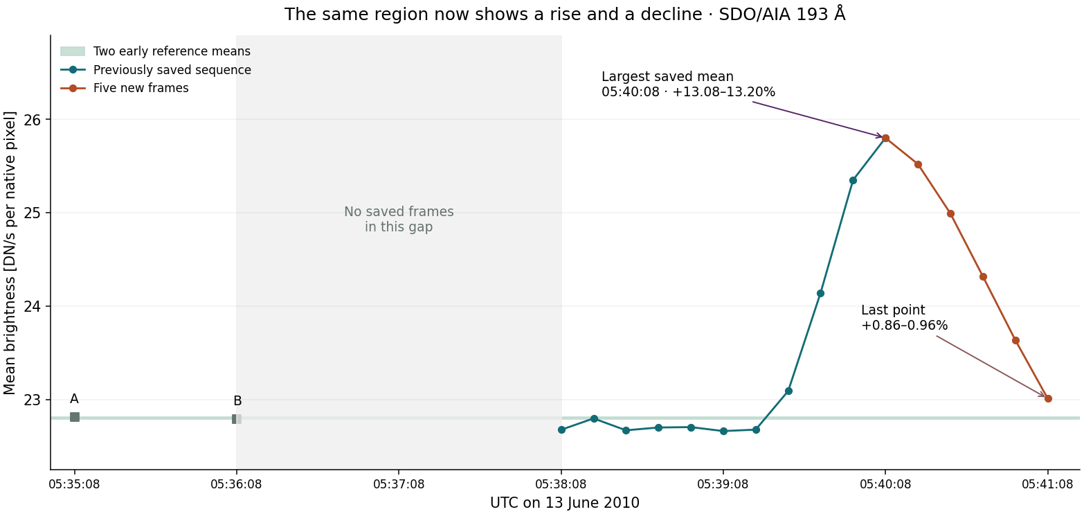
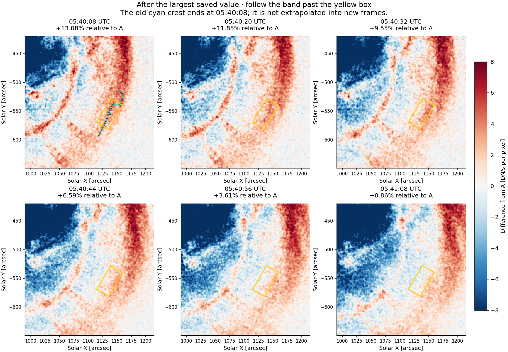
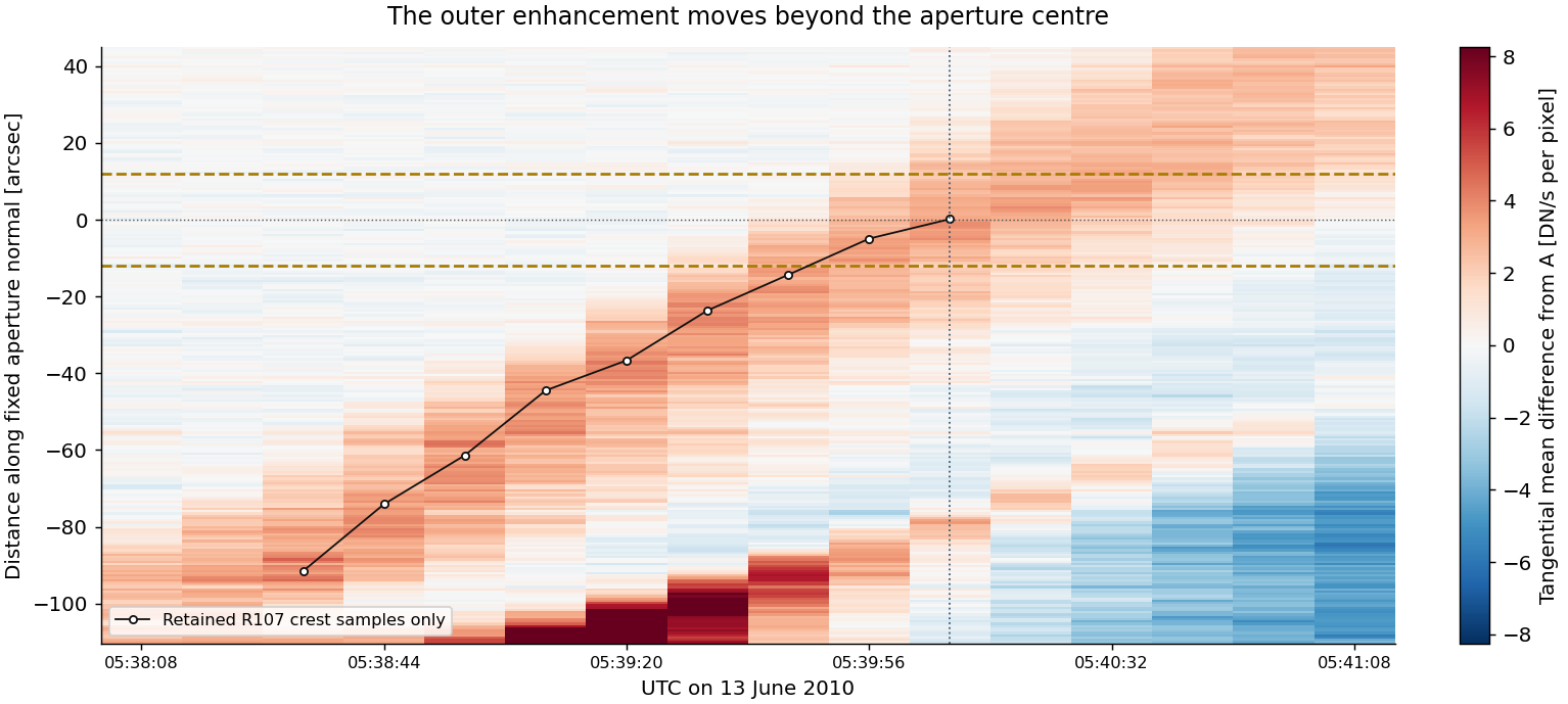
Supported: the main enhancement's passage to the outward side and a declining signal inside the same fixed aperture. Still open: a unique exit time, the end of the faint tail and a stable post-event level. A small positive mean can reflect remaining emission, changing background or instrumental/noise contributions; these are not separated here.
The largest sampled mean is 25.79895 DN/s per native pixel. Its excess above A/B is +2.98458 to +3.00759 DN/s per pixel. The last mean is 23.01030, still +0.19593 to +0.21894 DN/s per pixel above A/B. The mean therefore falls by 2.78865 DN/s per pixel over the next 60.01 s.
The largest sample at 05:40:08 lies between smaller samples at 05:39:56.07 and 05:40:20.08. This establishes a sampled turnover, not an exact continuous-time maximum or a statistical confidence interval. Five subsequent samples decline monotonically at the observed cadence.
As R115 showed, earlier science-frame fluctuations already exceed the A/B difference. We therefore do not equate the final 0.86–0.96% excess with zero, or assign a detection significance. The rise and fall remain a passband measurement; temperature, density and emitting depth can all affect EUV brightness.
| T_OBS UTC | Mean [DN/s per native pixel] | Change from A | Change from B | Pixels | Exposure [s] |
|---|---|---|---|---|---|
| 05:35:08.07 | 22.81437 | +0.00% | +0.10% | 3193 | 2.900862 |
| 05:36:08.09 | 22.79135 | -0.10% | +0.00% | 3192 | 2.900866 |
| 05:38:08.07 | 22.67517 | -0.61% | -0.51% | 3192 | 2.900863 |
| 05:38:20.07 | 22.79665 | -0.08% | +0.02% | 3193 | 2.900863 |
| 05:38:32.06 | 22.66954 | -0.63% | -0.53% | 3192 | 2.900865 |
| 05:38:44.07 | 22.69948 | -0.50% | -0.40% | 3193 | 2.900864 |
| 05:38:56.06 | 22.70379 | -0.48% | -0.38% | 3192 | 2.900863 |
| 05:39:08.07 | 22.66126 | -0.67% | -0.57% | 3193 | 2.900864 |
| 05:39:20.05 | 22.67675 | -0.60% | -0.50% | 3192 | 2.900868 |
| 05:39:32.08 | 23.09042 | +1.21% | +1.31% | 3193 | 2.900863 |
| 05:39:44.06 | 24.14063 | +5.81% | +5.92% | 3192 | 2.900870 |
| 05:39:56.07 | 25.34812 | +11.11% | +11.22% | 3193 | 2.900865 |
| 05:40:08.06 | 25.79895 | +13.08% | +13.20% | 3192 | 2.900866 |
| 05:40:20.08 | 25.51870 | +11.85% | +11.97% | 3193 | 2.900865 |
| 05:40:32.05 | 24.99212 | +9.55% | +9.66% | 3192 | 2.900864 |
| 05:40:44.07 | 24.31855 | +6.59% | +6.70% | 3193 | 2.900869 |
| 05:40:56.06 | 23.63740 | +3.61% | +3.71% | 3192 | 2.900866 |
| 05:41:08.07 | 23.01030 | +0.86% | +0.96% | 3193 | 2.900865 |
| Input | Origin | Category | Limit |
|---|---|---|---|
| Five new images and their metadata | Original SDO/AIA 193 Å FITS, public VSO/NSO delivery | MEASURED · this event | Detector brightness is not a direct density measurement. |
| Earlier thirteen means and images | Saved R115 record and arrays, reused exactly | DERIVED FROM EVENT DATA · retained | No repeat fit or retrospective change to earlier values. |
| Fixed box and early references | R112 main sky polygon; R114 references A and B | ANALYSIS CHOICE | Fixed sky region, not one fluid parcel. Background choice is not the total error. |
| Pointing | Same retained event-day calibration used in R113–R115 | SOURCE-DERIVED · instrument calibration | Residual alignment remains unmeasured. |
| New brightness means | Unsmoothed native pixel centres / exposure, averaged inside the same box | DERIVED FROM EVENT DATA · new result | Noise, scattering, thermal response and line-of-sight components remain unresolved. |
| Crest after 05:40:08 | No new positions assigned | UNRESOLVED quantitatively | The image sequence supports outward passage; no precise exit time is fitted. |
| Plasma parameters and wave type | No new values or labels assigned | UNRESOLVED | Earlier conditional RMO completions remain unchanged. |
| T_OBS UTC | Catalogue identifier | History |
|---|---|---|
| 05:35:08.07 | aia__lev1:193:1055482542 | Reused R115 original |
| 05:36:08.09 | aia__lev1:193:1055482602 | Reused R115 original |
| 05:38:08.07 | aia__lev1:193:1055482722 | Reused R115 original |
| 05:38:20.07 | aia__lev1:193:1055482734 | Reused R115 original |
| 05:38:32.06 | aia__lev1:193:1055482746 | Reused R115 original |
| 05:38:44.07 | aia__lev1:193:1055482758 | Reused R115 original |
| 05:38:56.06 | aia__lev1:193:1055482770 | Reused R115 original |
| 05:39:08.07 | aia__lev1:193:1055482782 | Reused R115 original |
| 05:39:20.05 | aia__lev1:193:1055482794 | Reused R115 original |
| 05:39:32.08 | aia__lev1:193:1055482806 | Reused R115 original |
| 05:39:44.06 | aia__lev1:193:1055482818 | Reused R115 original |
| 05:39:56.07 | aia__lev1:193:1055482830 | Reused R115 original |
| 05:40:08.06 | aia__lev1:193:1055482842 | Reused R115 original |
| 05:40:20.08 | aia__lev1:193:1055482854 | New R116 original |
| 05:40:32.05 | aia__lev1:193:1055482866 | New R116 original |
| 05:40:44.07 | aia__lev1:193:1055482878 | New R116 original |
| 05:40:56.06 | aia__lev1:193:1055482890 | New R116 original |
| 05:41:08.07 | aia__lev1:193:1055482902 | New R116 original |
Five new original FITS total 61,030,080 bytes. All have QUALITY = 0, MISSVALS = 0 and complete coverage of the main aperture. Byte counts, SHA-256 hashes, complete array reads and source identifiers were checked. All thirteen earlier means and image/strip arrays are unchanged.
The sky polygon, pointing algorithm, 0.6″ grid and native-pixel mean operator are the same as R115. Each quantitative sample is the unsmoothed level-1 detector value divided by its exposure. Negative values are retained. No empirical registration, new speed fit, PSF correction, thermal response fit or RMO calculation is added.
Images use bilinear sampling and Gaussian sigma 1.5 output pixels for display only. Original panels retain the same asinh limits; all difference panels retain ±8 DN/s. The time-distance strip retains its earlier separate scale and averages across the same 48″ tangential width. Original files are unchanged; exact headers, paths and source responses are retained with R116.
We now have a measured local brightness history with a rising and falling branch associated with the moving outer enhancement. This is a firmer temporal basis for comparing channels than one selected bright image. It does not establish a plasma compression, a unique temperature, a downstream plateau or MHD type. No earlier conditional RMO state is selected or rejected.
One proposed next bounded step: add three epochs in each of 171 and 211 Å: before the rise, during the decline and near the end of this 193 Å pulse. Reuse their existing early references and near-peak images. At most six new files would test whether the other channels follow the same local structure and time history. Their actual times remain separate; no simultaneous-ratio assumption or thermal fit is automatic. These files have not been requested in R116.
What we measured: a rise and decline of 193 Å brightness in the fixed patch. The largest saved excess is 13.08–13.20%; the final excess is 0.86–0.96%, depending on reference A or B. Real images show the main band moving outward past the region.
What we chose or assumed: the retained aperture and early references, the pointing calibration and the same brightness operator. The box is not a fluid parcel. Earlier radio and published thermal quantities have not become direct measurements of this patch.
What RMO says here: the image-based correspondence is supported over a rising and falling branch. R116 supplies no new MHD family identification; earlier conditional model completions remain conditional.
What remains ambiguous: density, temperature, emission depth, plasma flow, field direction and exact end of the faint signal. Full uncertainties and the spatial match of other diagnostics remain open.
What to measure next: a bounded 171/211 temporal comparison in this same region. This tests whether the other channel changes follow this pulse. It is the next practical correspondence step, not a demonstrated global ranking of all possible measurements.
This is an interim observer card. The event's final physical reconstruction is not yet complete.
Different events do not need the same diagnostics. RMO asks what the existing observations allow us to conclude, and which missing observable could distinguish the surviving alternatives.
Radio, spectroscopy, DEM/EUV, magnetic constraints and stereoscopy are optional routes with their own assumptions. No radio does not make an event unusable. Density and compression derived from the same radio lanes are not independent confirmations. A magnetic model or inferred temperature must also retain its assumptions and match to the selected patch.
The full protocol is saved as RMO_observational_protocol.md. The eventual event × diagnostics × outcome matrix will be built from checked event cards, with availability, matching and physical usefulness distinguished. An incomplete cell is a result to explain, not a reason to force a wave label.
The current catalogue has 11 cards, E01–E11: ten EUV event/study cases and one IRIS flare-loop comparison. The separate 13 February 2009 worked geometry example gives a proposed working pool of 12 records, not 12 equivalent solved events. E03 has no fixed date in its current card. E11, 13 June 2010, remains our detailed pilot.
After this pilot, use the same protocol for the remaining cards: saved evidence first, then one bounded missing-input question, with measured, event-derived and assumed inputs kept distinct. Full reconstruction is appropriate only where the data support it. Conditional and unresolved/control results also belong in the article. No other event is launched here.
The saved inventory is RMO_observational_pool_R116.md. It uses the corrected current E09 date, 22 June 2015. PDS cases, model tests, deferred searches and the 2017 demonstration movie do not silently increase this selected event count.
13 June 2010 · SDO/AIA 193 Å · the same PA116 region
The saved images support a link between the approaching outer enhancement and the rise in this fixed region. By the final frame, the mean brightness has increased by 13.08–13.20% relative to the two early references. The crest is still inside the box, and the final point is still rising.
We have the approach and entry, but not the complete passage. There is no later frame here to show a maximum, decline or exit. This is a measured passband brightness change; it does not yet give the density jump or a fast/slow identification.
Yellow is the fixed measurement box. Cyan is the previously saved crest, with a dot at the central estimate. Left: original image. Right: difference from reference A. The image scales stay fixed throughout.
119.98 s since previous saved frame.
Original images: SDO/AIA. Play advances through the eleven science frames, one saved frame every 0.7 s; this is not real-time motion. Use the slider to inspect the two earlier references. Actual observation times and gaps are always shown. No invented intermediate frames.
| UTC | Brightness change using A or B | Central crest offset | Position relative to the box |
|---|---|---|---|
| 05:39:20.05 | -0.60% to -0.50% | -36.65″ | Before the inner edge |
| 05:39:32.08 | +1.21% to +1.31% | -23.62″ | Before the inner edge |
| 05:39:44.06 | +5.81% to +5.92% | -14.32″ | Before the inner edge |
| 05:39:56.07 | +11.11% to +11.22% | -4.90″ | Inside the box |
| 05:40:08.06 | +13.08% to +13.20% | +0.19″ | Inside the box |
The offset is measured along the saved image-plane normal: the inner edge is −12″, the centre is 0″ and the outer edge is +12″. Percentage ranges come only from choosing A or B; they are not 1σ errors or a full uncertainty interval.
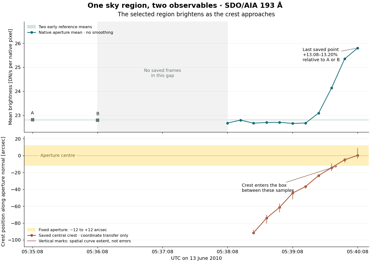
From 05:39:20 to the last frame, the means rise from 22.677 to 25.799 DN/s per native pixel. At 05:39:32 the change is already positive relative to both references, although the central crest is still outside the box. A feature with finite width can affect an aperture before its crest enters it; this does not establish the first physical arrival time.
The central saved crest lies before the inner edge at 05:39:44.06 and inside at 05:39:56.07 UTC. These samples are 12.01 s apart. Part of the curved crest already overlaps the box in the earlier of these frames, so there is no single entry time for the entire curve.
This is a sampled geometric bracket, not a ±6 s measurement error. The crest is an estimate from smoothed log-ratio images; its method uncertainty, residual registration and the front's finite width have not been converted into a complete timing uncertainty. The leading edge, brightness onset and crest are different observables.
The last-frame central coincidence is expected: R112 placed the box around the saved final crest. That coincidence is not an independent validation. The new evidence is the preceding brightness history and the visible approach into the same fixed region.
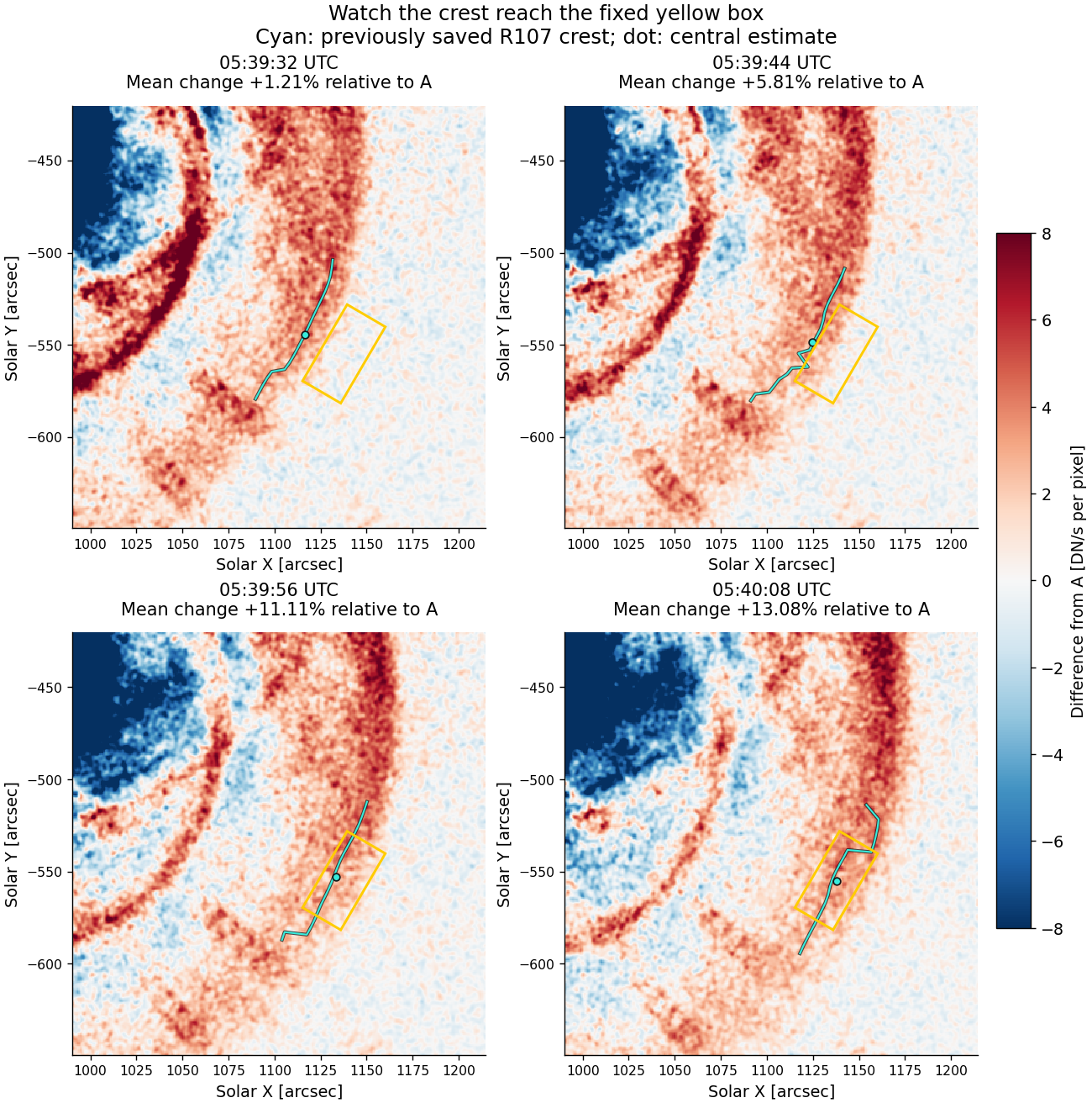
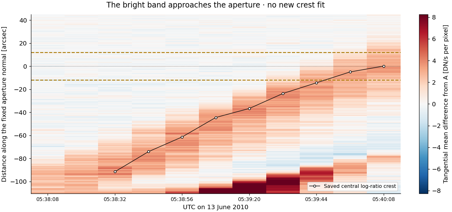
| T_OBS UTC | Mean [DN/s per native pixel] | Change from A | Change from B | Central crest offset | Native pixels |
|---|---|---|---|---|---|
| 05:35:08.07 | 22.81437 | +0.000% | +0.101% | Not tracked | 3193 |
| 05:36:08.09 | 22.79135 | -0.101% | +0.000% | Not tracked | 3192 |
| 05:38:08.07 | 22.67517 | -0.610% | -0.510% | Not tracked | 3192 |
| 05:38:20.07 | 22.79665 | -0.078% | +0.023% | Not tracked | 3193 |
| 05:38:32.06 | 22.66954 | -0.635% | -0.534% | -91.55″ | 3192 |
| 05:38:44.07 | 22.69948 | -0.504% | -0.403% | -74.10″ | 3193 |
| 05:38:56.06 | 22.70379 | -0.485% | -0.384% | -61.38″ | 3192 |
| 05:39:08.07 | 22.66126 | -0.671% | -0.571% | -44.47″ | 3193 |
| 05:39:20.05 | 22.67675 | -0.603% | -0.503% | -36.65″ | 3192 |
| 05:39:32.08 | 23.09042 | +1.210% | +1.312% | -23.62″ | 3193 |
| 05:39:44.06 | 24.14063 | +5.813% | +5.920% | -14.32″ | 3192 |
| 05:39:56.07 | 25.34812 | +11.106% | +11.218% | -4.90″ | 3193 |
| 05:40:08.06 | 25.79895 | +13.082% | +13.196% | +0.19″ | 3192 |
Before the sustained late rise, the science-frame means span 22.6613–22.7967 DN/s per pixel. They differ from A by about −0.67% to −0.08%. These variations are larger than the 0.10% separation of the two early reference means. Thus R114's two-reference comparison must not be read as a bound on all later fluctuations. This stage does not separate solar background changes from noise or residual alignment.
The final excess is +2.98458 to +3.00759 DN/s per native pixel, or +13.082% to +13.196%. These are two reference choices for one measurement. No 1σ/2σ/3σ interval, density jump or temperature estimate is assigned.
The two early references are 60.02 s apart. There is then a 119.98 s gap before the eleven science frames, spaced about 12 s apart. No behaviour inside the gaps or after the last sample is observed here.
| Input | Origin | Category | What remains open |
|---|---|---|---|
| Images, exposure times and quality | 13 original SDO/AIA 193 Å FITS, already saved | MEASURED · event data | Detector brightness is not density or compression. |
| Fixed 24″ × 48″ sky box | R112, centred on the saved final-frame crest | ANALYSIS CHOICE using saved geometry | Last-frame central coincidence is expected by construction. |
| Crest positions | R107 log-ratio crest, transferred through the same detector pixels | DERIVED FROM EVENT DATA · retained result | Brightness crest, not a unique shock boundary. No new speed fit. |
| Pointing calibration | The retained event-day master pointing table used in R113/R114 | SOURCE-DERIVED · instrument calibration | Residual registration error has not been measured. |
| Brightness means and differences | Unsmoothed native samples divided by their own exposure, within the same polygon | DERIVED FROM EVENT DATA · new R115 result | Noise, scattering and changing line-of-sight emission remain unseparated. |
| Reference A and B | 05:35:08.07 and 05:36:08.09 UTC, retained from R114 | ANALYSIS CHOICE · two candidate early references | Their difference is not a bound on later background variation. |
| Temperature, density, plasma flow and field | No new values are assigned in this stage | UNRESOLVED | The earlier conditional RMO states are unchanged. |
| T_OBS UTC | Catalogue identifier | Exposure [s] | QUALITY / MISSVALS |
|---|---|---|---|
| 05:35:08.07 | aia__lev1:193:1055482542 | 2.900862 | 0 / 0 |
| 05:36:08.09 | aia__lev1:193:1055482602 | 2.900866 | 0 / 0 |
| 05:38:08.07 | aia__lev1:193:1055482722 | 2.900863 | 0 / 0 |
| 05:38:20.07 | aia__lev1:193:1055482734 | 2.900863 | 0 / 0 |
| 05:38:32.06 | aia__lev1:193:1055482746 | 2.900865 | 0 / 0 |
| 05:38:44.07 | aia__lev1:193:1055482758 | 2.900864 | 0 / 0 |
| 05:38:56.06 | aia__lev1:193:1055482770 | 2.900863 | 0 / 0 |
| 05:39:08.07 | aia__lev1:193:1055482782 | 2.900864 | 0 / 0 |
| 05:39:20.05 | aia__lev1:193:1055482794 | 2.900868 | 0 / 0 |
| 05:39:32.08 | aia__lev1:193:1055482806 | 2.900863 | 0 / 0 |
| 05:39:44.06 | aia__lev1:193:1055482818 | 2.900870 | 0 / 0 |
| 05:39:56.07 | aia__lev1:193:1055482830 | 2.900865 | 0 / 0 |
| 05:40:08.06 | aia__lev1:193:1055482842 | 2.900866 | 0 / 0 |
All thirteen originals were already saved; R115 downloaded nothing. Their hashes match the previous records. Original files are unchanged and all main-aperture pixels are finite. Exact source paths, hashes, headers and samples are saved in R115_timing_record.json and the accompanying arrays.
A catalogue record identifies an observation. Its FITS file contains the image and header. The same R114 mean operator is used: unsmoothed native pixel centres inside the fixed R112 sky polygon, divided by their own exposure time. The A, B and final means reproduce R114 numerically.
The old R107 crest coordinates are passed through the original WCS to detector pixels, then through the same R113 pointing update. This changes the displayed crest coordinates by about 0.19–0.20″ and does not refit its speed. That shift is a calibration change, not a residual-alignment error estimate. The sky polygon itself stays fixed.
Displayed images use bilinear 0.6″ sampling and Gaussian sigma 1.5 output pixels. Differences use a fixed ±8 DN/s scale to show the outer enhancement; stronger inner structures clip. The original images also share one fixed asinh scale. No display clipping or smoothing enters the native means. The time-distance strip uses unsmoothed bilinear samples averaged across 48″; its colour scale differs from the image panels.
No time interpolation, new ridge selection, empirical alignment, PSF correction, thermal response model or plasma diagnosis is added. Calibration references remain the documented pointing transformation and the saved event-day master pointing table in R113.
Supported: a spatially and temporally matched brightness increase during the approach and initial entry of the selected outer enhancement. The two retained references give the same late-rise interpretation.
Not established: complete passage, a downstream plateau, a unique emitting plasma component, compression, temperature, field strength or MHD type. None of the earlier conditional RMO states is selected or rejected. This is a correspondence check within the same images, not an independent validation of the tracking method.
One next bounded step: obtain at most the five next 193 Å frames near 05:40:20–05:41:08 UTC and inspect whether the signal reaches a maximum, declines and clears the aperture. Keep the same aperture and references. If those frames still do not cover the end, report that limit; do not automatically expand the download or begin a thermal fit. These new frames have not been requested in R115.
13 June 2010 · the same PA116 sky region
The sign of the change survives both selected references: 171 Å becomes fainter, while 193 and 211 Å become brighter. In these three bands, the effect of choosing reference A or B is small for the measured aperture mean. The weak 335 Å signal needs more care.
R114 answers one limited question. We compared two early frames, A and B, one minute apart, with the retained later frame E in each channel. This checks the effect of choosing between these two backgrounds. It does not supply a full error budget or identify a shock type.
| Channel | Early B versus A | Later change using either reference | Effect of choosing A or B | Interpretation |
|---|---|---|---|---|
| 171 Å | +0.04% | Decrease | ±0.26% of the change | Same sign for A and B; small reference-choice effect |
| 193 Å | -0.10% | Increase | ±0.38% of the change | Same sign for A and B; small reference-choice effect |
| 211 Å | -0.31% | Increase | ±0.45% of the change | Same sign for A and B; small reference-choice effect |
| 335 Å | +7.10% | Increase | ±12.39% of the change | Weak signal: noise and calibration still needed |
“Early B versus A” is 100 × (B−A)/A. The ± column is half the two-reference range divided by its midpoint magnitude. These columns use different denominators. All values use the declared native-pixel aperture mean; they are not statistical uncertainties.
Start with 193 Å, then open another channel. A is near 05:35 UTC, B near 05:36 UTC, and E near 05:40 UTC. Exact times differ between channels and are listed below.
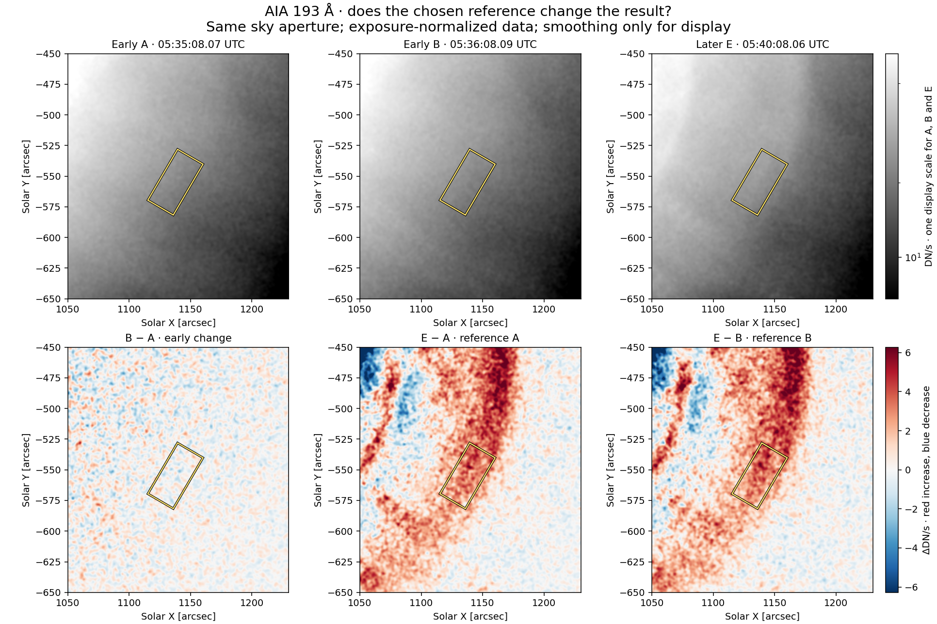
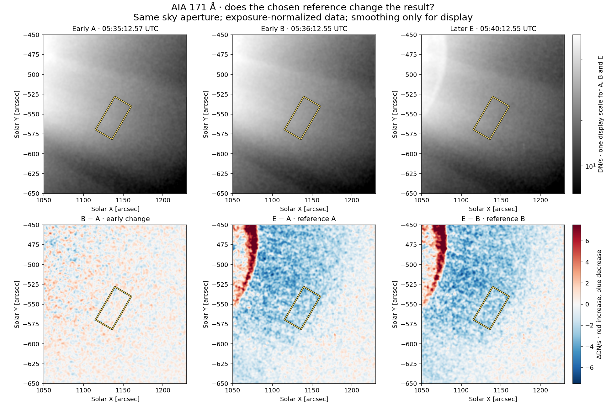
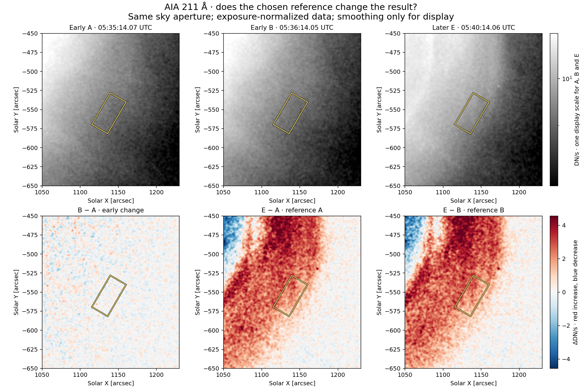
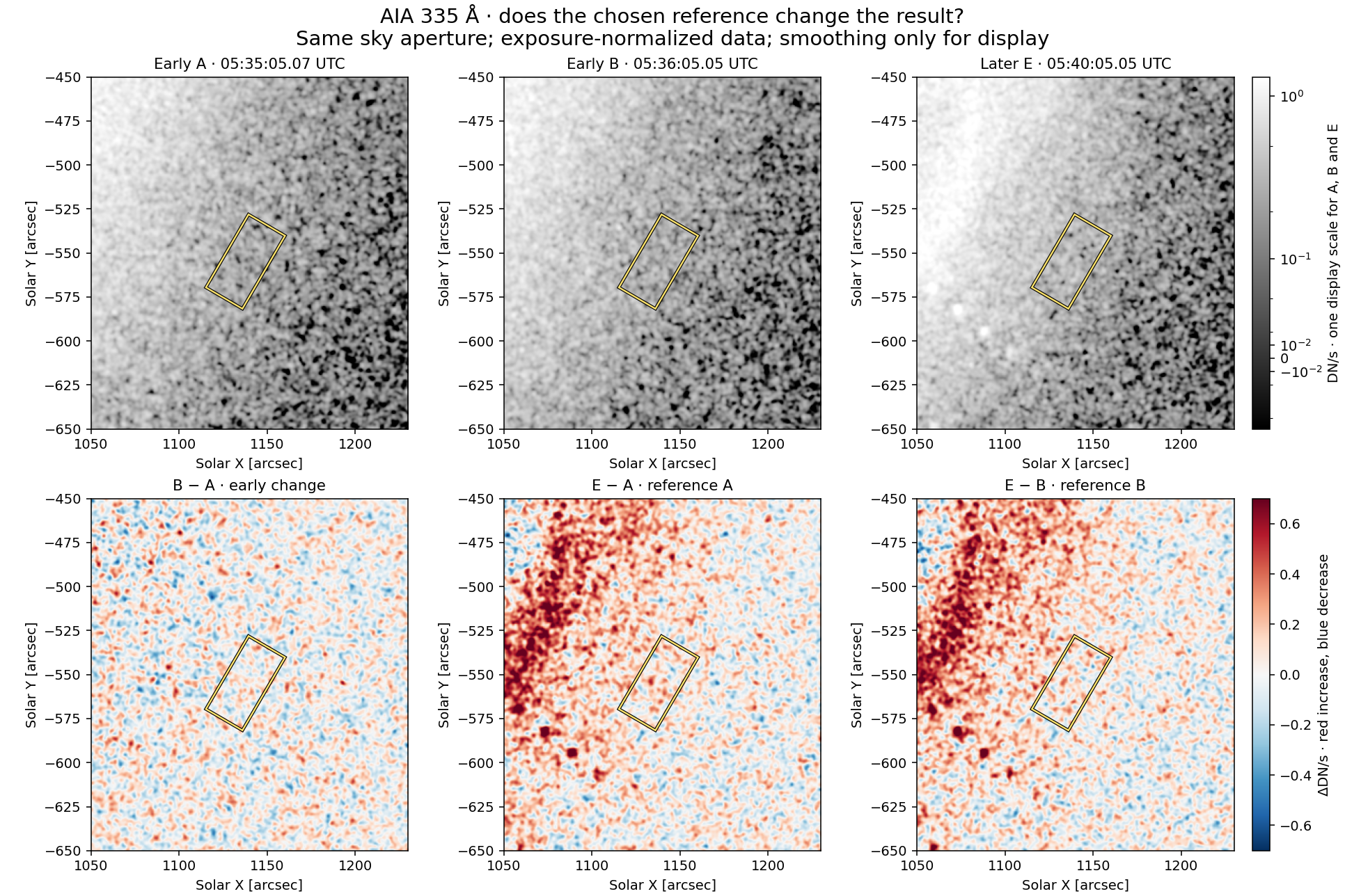
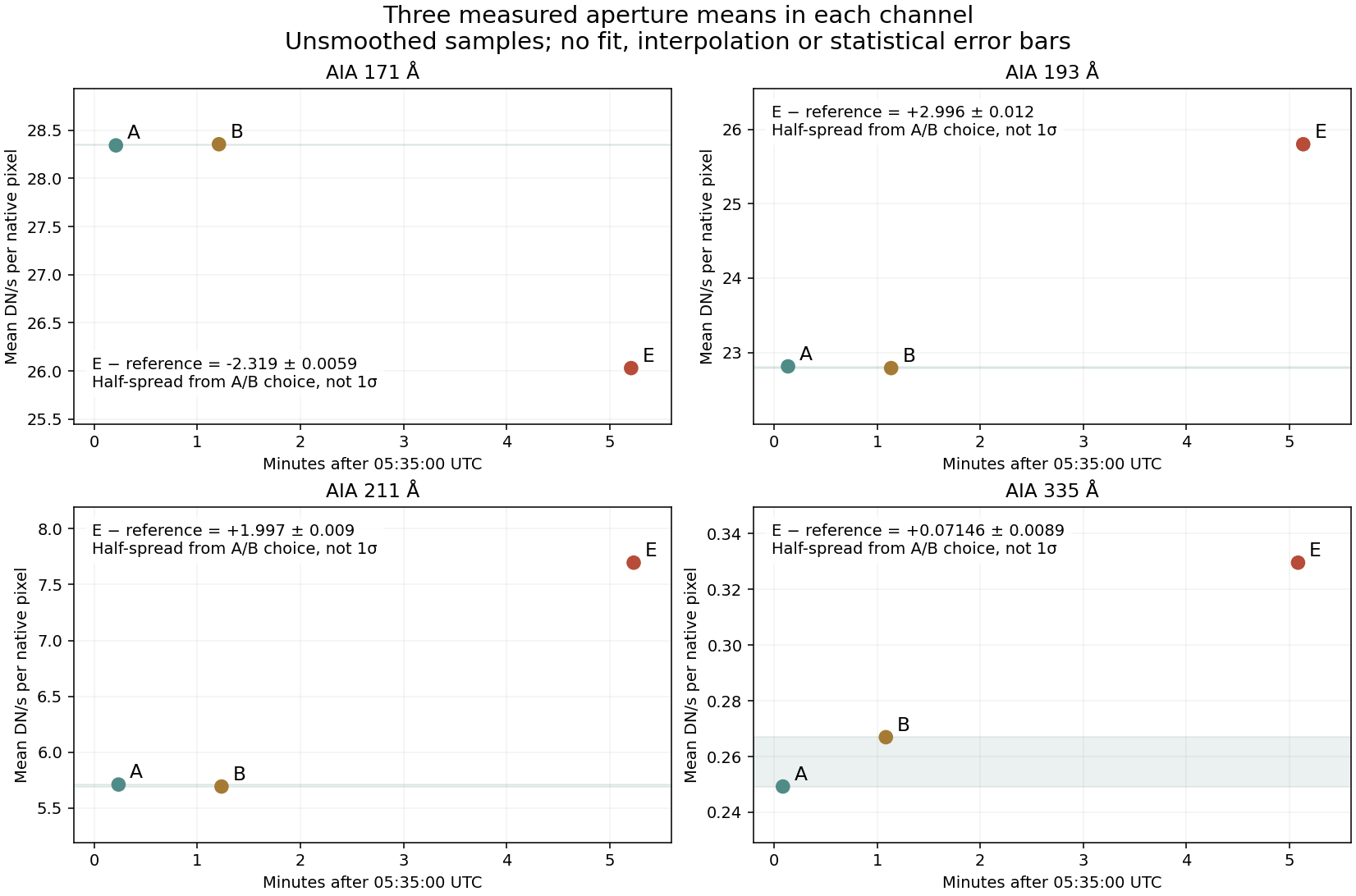
Units: DN/s per native pixel. DN means detector counts. For the values below, we divide each unsmoothed level-1 pixel by its exposure time and average native pixel centres inside the saved sky polygon. The images are smoothed for viewing; these numbers are not.
| Channel | Early A | Early B | Later E | E − A | E − B | Midpoint ± half-spread |
|---|---|---|---|---|---|---|
| 171 Å | 28.34315 | 28.35503 | 26.02969 | -2.31346 | -2.32533 | -2.31940 ± 0.00594 |
| 193 Å | 22.81437 | 22.79135 | 25.79895 | +2.98458 | +3.00759 | +2.99609 ± 0.01151 |
| 211 Å | 5.70887 | 5.69094 | 7.69670 | +1.98783 | +2.00576 | +1.99679 ± 0.00897 |
| 335 Å | 0.24924 | 0.26694 | 0.32955 | +0.08031 | +0.06261 | +0.07146 ± 0.00885 |
For example, the 193 Å change is +2.99609 ± 0.01151 DN/s per pixel when we summarize only the two possible reference choices. The corresponding relative half-spread is ±0.38%. For 335 Å it is +0.07146 ± 0.00885 DN/s per pixel, or ±12.39%.
These are not 1σ errors. They omit detector noise, residual alignment, PSF/scattered light, background evolution outside the sampled times and calibration uncertainty. No claim of sub-percent measurement accuracy is made.
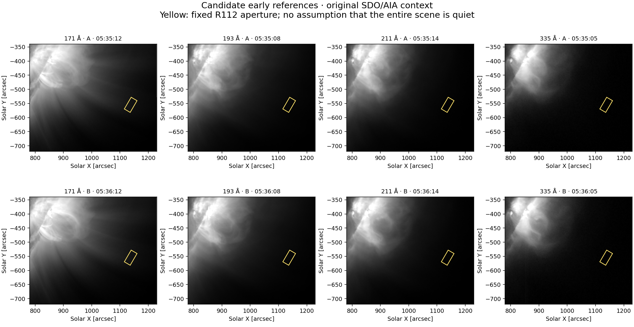
The early local means differ by +0.042%, −0.101% and −0.314% in 171, 193 and 211 Å. Their early difference maps lack a comparably strong coherent band at the fixed displayed scales. This supports using either image for a provisional local difference comparison.
Two samples cannot certify an uncontaminated pre-event background, rule out transient changes between them, or show how the background evolves over the next four minutes. No long backward extrapolation of the front speed is used to declare the images clean. The 335 Å early mean changes by +7.10%; detector noise and other contributions have not been separated.
| Channel | Epoch | T_OBS UTC | Exposure [s] | Native aperture pixels |
|---|---|---|---|---|
| 171 Å | A | 05:35:12.57 | 2.900827 | 3207 |
| 171 Å | B | 05:36:12.55 | 2.900822 | 3207 |
| 171 Å | E | 05:40:12.55 | 2.900827 | 3207 |
| 193 Å | A | 05:35:08.07 | 2.900862 | 3193 |
| 193 Å | B | 05:36:08.09 | 2.900866 | 3192 |
| 193 Å | E | 05:40:08.06 | 2.900866 | 3192 |
| 211 Å | A | 05:35:14.07 | 2.901267 | 3192 |
| 211 Å | B | 05:36:14.05 | 2.901271 | 3192 |
| 211 Å | E | 05:40:14.06 | 2.901269 | 3192 |
| 335 Å | A | 05:35:05.07 | 2.901402 | 3193 |
| 335 Å | B | 05:36:05.05 | 2.901400 | 3193 |
| 335 Å | E | 05:40:05.05 | 2.901405 | 3193 |
All 12 files are fully readable, with QUALITY = 0 and MISSVALS = 0; every main aperture is fully covered. The two early times are separated by 59.98–60.02 s within a band. The later frame follows them by about five and four minutes. Channels remain asynchronous; no cross-channel intensity ratio or time interpolation was made.
The original 12 AIA193 files and the three R113 additions are unchanged. This stage acquired seven files (73,255,680 bytes) and reused five. Source hashes match the verified saved files.
| Input | Where it comes from | Category | Limit |
|---|---|---|---|
| Original samples and times | The 12 identified AIA files below | MEASURED · calibrated level-1 detector samples and metadata | DN are detector units; no temperature or density follows directly. |
| Pointing update | Same event-day 03:00–06:00 master pointing row used in R113 | SOURCE-DERIVED · instrument calibration | A metadata correction does not give the remaining alignment error. |
| Aperture | Saved R112 polygon: X = 1137.700″, Y = −554.893″; 24″ × 48″ | ANALYSIS CHOICE using saved geometry | Fixed sky region, not a tracked fluid parcel. |
| Reference A and B | Two cycles near 05:35 and 05:36, chosen before inspecting brightness | ANALYSIS CHOICE · candidate pre-front reference | Two samples do not prove stability between them or through the following four minutes. |
| Reported ± values | Half of the difference between E−A and E−B | DERIVED from the two selected references | This is not 1σ, 2σ, 3σ or a total uncertainty. |
| Temperature, density, compression, magnetic field | No new values adopted in R114 | UNRESOLVED | Earlier conditional RMO states remain unchanged. |
A catalogue record identifies a selected observation. The FITS file contains its image and header. The following identifiers let us trace every value back to its file.
| Band / epoch | Catalogue identifier | File history | Origin |
|---|---|---|---|
| 171 Å / A | aia__lev1:171:1055482547 | New original FITS via VSO/NSO | MEASURED · instrument data |
| 171 Å / B | aia__lev1:171:1055482607 | New original FITS via VSO/NSO | MEASURED · instrument data |
| 171 Å / E | aia__lev1:171:1055482847 | Reused original FITS | MEASURED · instrument data |
| 193 Å / A | aia__lev1:193:1055482542 | Reused original FITS | MEASURED · instrument data |
| 193 Å / B | aia__lev1:193:1055482602 | New original FITS via VSO/NSO | MEASURED · instrument data |
| 193 Å / E | aia__lev1:193:1055482842 | Reused original FITS | MEASURED · instrument data |
| 211 Å / A | aia__lev1:211:1055482548 | New original FITS via VSO/NSO | MEASURED · instrument data |
| 211 Å / B | aia__lev1:211:1055482608 | New original FITS via VSO/NSO | MEASURED · instrument data |
| 211 Å / E | aia__lev1:211:1055482848 | Reused original FITS | MEASURED · instrument data |
| 335 Å / A | aia__lev1:335:1055482539 | New original FITS via VSO/NSO | MEASURED · instrument data |
| 335 Å / B | aia__lev1:335:1055482599 | New original FITS via VSO/NSO | MEASURED · instrument data |
| 335 Å / E | aia__lev1:335:1055482839 | Reused original FITS | MEASURED · instrument data |
The pointing algorithm, master table and 0.6″ sky grid are the same as R113. Files remain unchanged; copied headers are used for WCS sampling. No empirical shift was fitted. Unsampled detector-edge values stay missing; negative level-1 values remain. Negative counts do not mean negative physical emission.
Original comparison images share their contrast scale across A/B/E within each band. The three differences share symmetric limits within each band. Display Gaussian sigma is 1.5 output pixels; quantitative means use unsmoothed native samples. The CSV and JSON also record a common-grid mean as a processing comparison: it preserves all four change signs, but is not an independent measurement. No pixel-independence assumption or error on the mean is inferred from spatial scatter.
Pointing transformation · VSO data access and mirror selection. Exact source URLs, hashes, requests, masks, arrays and scripts are saved with R114.
Ready: a real local brightness-change measurement whose sign is unchanged by the two selected early references. For 171/193/211 Å, changing between these references has a small effect under the stated averaging method.
Still open: the total uncertainty, the time history tying this signal to the tracked front, and a physically justified thermal interpretation. Passband brightening is not a density jump, and 171 Å fading is not a unique temperature or mass-loss diagnosis. No conditional RMO state has been rejected or selected.
One next bounded step: use the already saved 193 Å sequence to compare the aperture's brightness change with the previously tracked front position, retaining the R107 geometry and speed fit. Determine what part of the front's approach/passage is actually covered before choosing any further data or a thermal fit. No new downloads are needed to start that step, and it has not been run here.
13 June 2010 · PA116 outer-front region
The R113 image and timing check is complete. All four selected AIA files are now available and fully readable. The same fixed sky aperture is covered in every channel. This closes the one-epoch inspection; it does not yet establish one common emitting front or a temperature.
What matters for the next measurement: the four T_OBS values span 9.01 s. The 335 Å values in our aperture are very low. Before using channel brightnesses to constrain the plasma, we need a checked pre-front reference and the local change through time.
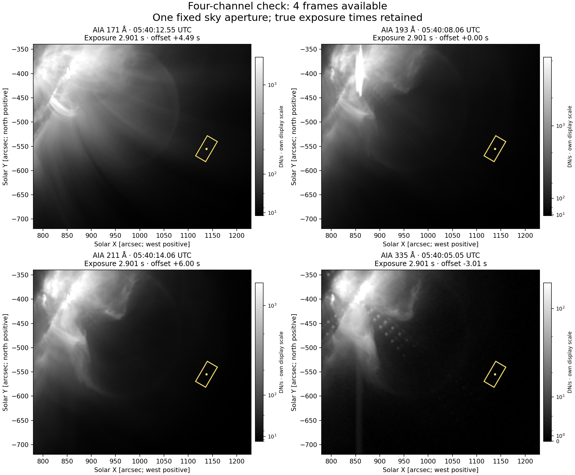
| Channel | T_OBS UTC | Exposure | Offset from 193 Å |
|---|---|---|---|
| 171 Å | 05:40:12.55 | 2.900827 s | +4.49 s |
| 193 Å | 05:40:08.06 | 2.900866 s | +0.00 s |
| 211 Å | 05:40:14.06 | 2.901269 s | +6.00 s |
| 335 Å | 05:40:05.05 | 2.901405 s | -3.01 s |
These offsets are recorded time differences, not ± uncertainties or sigma errors. In order of T_OBS: 335, 193, 171, 211 Å. The 171 and 211 Å exposures partly overlap; the set is not simultaneous. Exposure durations are about 2.901 s. Header midpoint rounding agrees within 0.001 s; this does not certify clock accuracy.
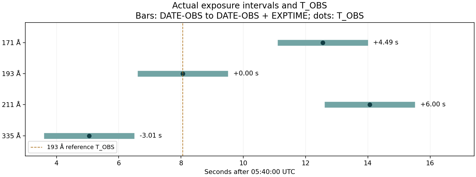
The unchanged R107 mean image-normal speed gives a motion scale of 8.63″ across 9.01 s, about 36% of the aperture's chosen 24″ normal width. This estimates the importance of timing; it is not a new displacement measurement, speed fit or confidence bound.
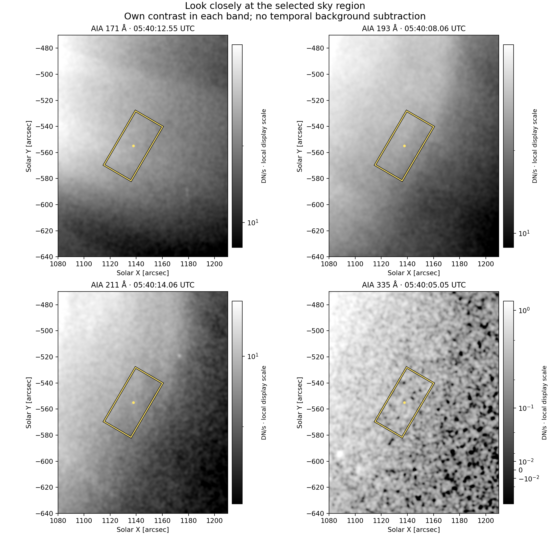
Structures are visible in 171, 193 and 211 Å. The 335 Å local view is grainy and its native aperture values range from −3 to +6 DN; 477 of 3193 pixel values (14.9%) are negative. The negative values are retained. They do not represent negative physical emission.
This is not a non-detection limit or a rejection of hot plasma. A noise model, instrumental response and background are needed for those conclusions. One image per channel cannot isolate the changing outer front from the existing corona, nor prove that all channels sample the same plasma.
| Channel | Finite native pixels in aperture | Native value range | Negative values | Anchor coordinate change |
|---|---|---|---|---|
| 171 Å | 3207 | 43 to 111 DN | 0 | 0.358″ |
| 193 Å | 3192 | 48 to 104 DN | 0 | 0.190″ |
| 211 Å | 3192 | 9 to 39 DN | 0 | 0.258″ |
| 335 Å | 3193 | -3 to 6 DN | 477 | 0.284″ |
All four full frames have QUALITY = 0, MISSVALS = 0 and readable 4096 × 4096 arrays. The main aperture is fully covered and no selected pixel reaches the full-frame maximum of 16383 DN. Saturated pixels elsewhere in the images remain present; scattered light and PSF contamination have not been excluded.
The pointing transformation follows the documented aiapy header algorithm, followed by Astropy WCS and bilinear sampling on one 0.6″ grid. The original FITS bytes are retained. This is not a claim of running the full level-1.5 pipeline.
The final column is the change caused by updating the pointing metadata, not residual registration error, a ± bound or 1σ. No cross-channel feature shift was fitted. The wider 171 Å context has 950 missing grid points outside detector coverage; the main aperture is unaffected. The other three context grids are fully covered.
| Input | Value or source | Origin | Meaning and limits |
|---|---|---|---|
| 171 Å instrument data | aia__lev1:171:1055482847 | MEASURED · original SDO/AIA level-1 FITS | Wavelength, time, exposure, counts and quality from the file; counts are not plasma density or temperature. |
| 193 Å instrument data | aia__lev1:193:1055482842 | MEASURED · original SDO/AIA level-1 FITS | Wavelength, time, exposure, counts and quality from the file; counts are not plasma density or temperature. |
| 211 Å instrument data | aia__lev1:211:1055482848 | MEASURED · original SDO/AIA level-1 FITS | Wavelength, time, exposure, counts and quality from the file; counts are not plasma density or temperature. |
| 335 Å instrument data | aia__lev1:335:1055482839 | MEASURED · original SDO/AIA level-1 FITS | Wavelength, time, exposure, counts and quality from the file; counts are not plasma density or temperature. |
| Pointing calibration | Event-day 03:00–06:00 UTC master pointing row; documented LMSAL copy | SOURCE-DERIVED · instrument calibration | The coordinate changes below do not measure residual alignment uncertainty. |
| Sky aperture | X = 1137.700″; Y = −554.893″; 24″ × 48″ | ANALYSIS CHOICE · unchanged R112 polygon | The centre uses saved R106 geometry. The box is fixed on the sky; it is not a tagged plasma parcel. |
| Motion scale | Saved R107 mean image-normal rate; no new fit | SOURCE-DERIVED · earlier analysis of this event | Used only to show the scale of time offsets. It is not the plasma speed or an error bound. |
| Temperature, compression, B and field angle | No new estimates | UNRESOLVED in this stage | R110 conditional states and the R111 decision remain unchanged. |
Three new selected FITS total 30,530,880 bytes. The earlier 12 AIA193 files are unchanged. The 335 Å file was delivered through the original VSO route. After one 211 Å local copy failed the post-write integrity check, the same selected record was retrieved from the VSO NSO mirror and verified. The rejected bytes were never used for image analysis. Requests, source URLs, hashes and failures are preserved.
Counts are divided by EXPTIME and sampled bilinearly using the updated WCS. Gaussian smoothing, sigma = 1.5 output pixels, and separate asinh stretches are used only for display. Negative values remain in the data. Missing detector-edge values remain missing. No temporal interpolation, background subtraction, PSF/degradation correction, channel ratio, light curve or thermal fit was applied.
The original files contain two nonstandard NaN overscan header cards. Readable header exports use Astropy's serialization; source FITS bytes are unchanged. Full decompression and source hashes were checked separately.
Documented VSO mirror selection. Source records: R113_epoch_record.json, source/, results/; reproducible inspection: inspect_epoch.py.
Ready: four identified, readable files; exact exposure times; a shared sky grid; full coverage of the chosen aperture; an explicit record of origin and processing.
Still open: a stable pre-front reference, the evolving signal in this aperture, residual registration, and the physical correspondence between channel emission and plasma pressure. No R110 state is selected or rejected.
Next bounded step: compare two pre-front reference epochs within the already planned 05:35–05:37 UTC window in these same four channels and this same aperture. Test whether the background is stable enough for a local brightness-change measurement, with particular care for 335 Å. Those additional frames have not been acquired here.
Why this matters: an independent local thermal constraint can test conditional RMO states only after the observable is matched in position, time and background. This stage establishes the image inputs and identifies the remaining observational limits; it does not establish a temperature or a unique fast/slow classification.
13 June 2010 · preparation for a matched temperature test
The four-channel catalogue coverage is present. We found 161 AIA records between 05:35 and 05:43 UTC. We also defined a fixed aperture at our saved outer-crest position. This is a measurement plan, not a temperature result.
R112 decision: proceed first to a small four-band image check at one epoch. Confirm the actual times, pointing and local signal before acquiring the longer sequence. No magnetic-field or temperature bound has been added.
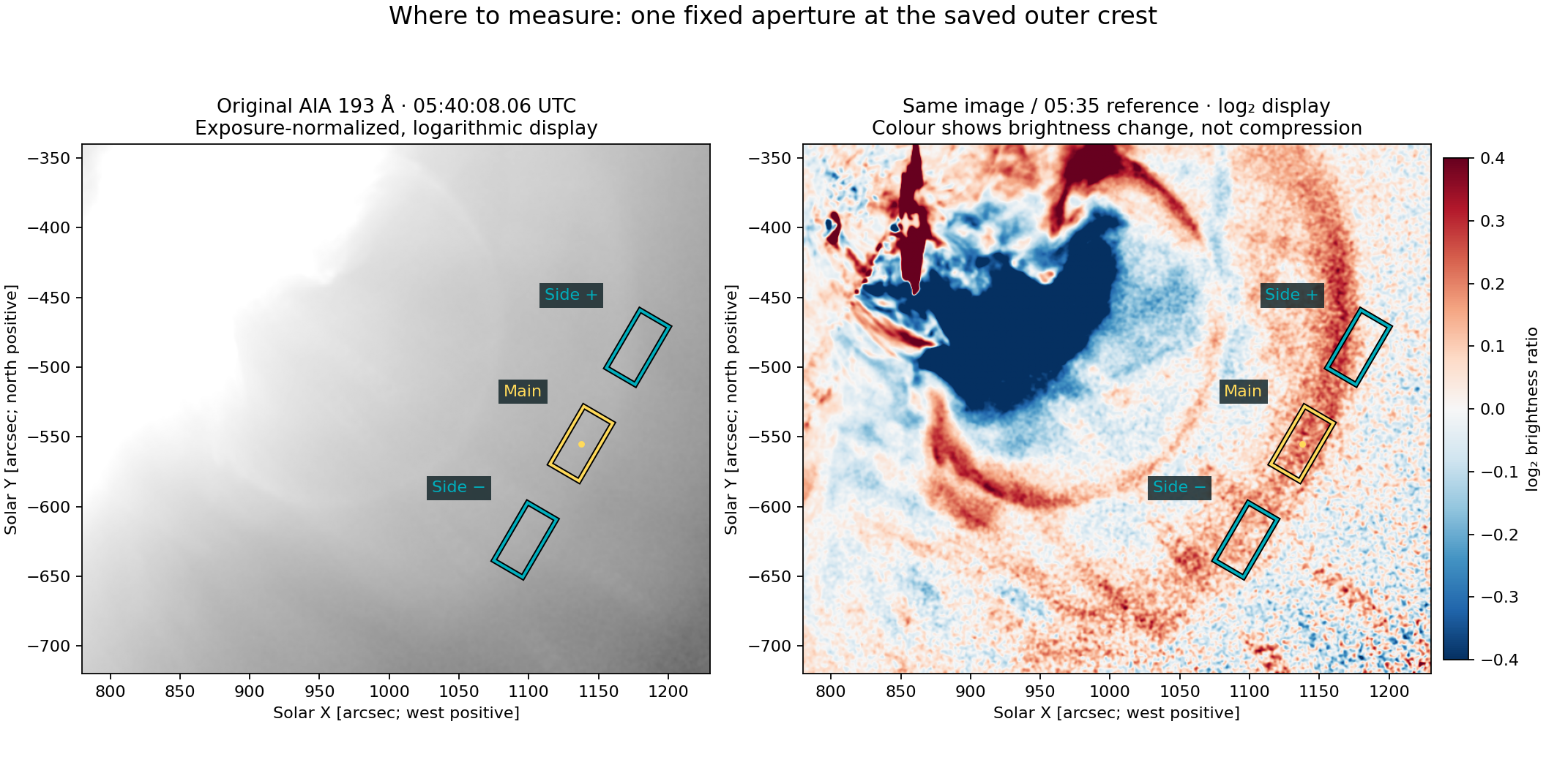
| Channel | Catalogue records | Catalogue spacing | Data available in the project |
|---|---|---|---|
| 171 Å | 40 | 12 s | Catalogue only; FITS not yet acquired |
| 193 Å | 40 | 12 s | 12 original FITS saved |
| 211 Å | 41 | 12 s | Catalogue only; FITS not yet acquired |
| 335 Å | 40 | 12 s | Catalogue only; FITS not yet acquired |
Catalogue records establish coverage. They do not certify file delivery, local signal quality or alignment between channels. The 211 Å count includes the query endpoint at 05:43:00.
| Quantity | Value | Where it comes from |
|---|---|---|
| Main aperture centre | X = 1137.700″; Y = −554.893″ | Saved image-based R106 crest estimate at 05:40:08.06 UTC; X west and Y north. |
| Aperture size | 24″ across the front; 48″ along it | Analysis choice. Not a measured front thickness or plasma volume. |
| Aperture orientation | Image-plane normal PA = 120.277° | Saved R106 diagnostic estimate. No new 3D normal or magnetic angle. |
| Pixel mask | 3191 native pixel centres; all finite | Checked using the saved 193 Å FITS WCS. Must be mapped separately in other bands. |
| Proposed temporal reference | 05:35–05:37 UTC, same aperture | Candidate pre-arrival interval. Per-channel background stability remains to be checked. |
| Side apertures | ±80″ along the tangent | Comparison regions. The front can also pass through them, so they are not automatically subtracted. |
The aperture stays fixed in the image plane. It does not follow a single moving parcel of plasma. The useful post-front interval must be separated from later CME passage using the images.
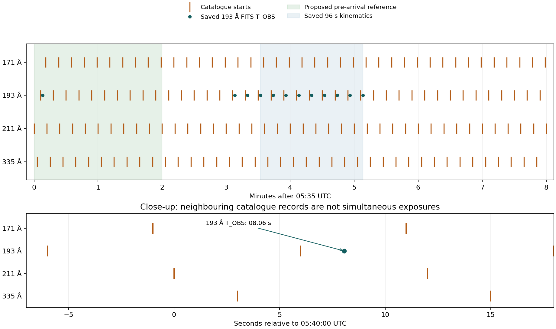
Nearest catalogue starts are displaced from the 193 Å starts by +5 s in 171 Å, −3 s in 335 Å, and either −6 or +6 s in 211 Å. The two 211 Å options are equally near in the catalogue. These are timing offsets, not error bars.
Using our already saved mean image speed, six seconds corresponds to about 5.7″ of normal pattern motion. A 24″-wide aperture has a crossing-time scale of about 25 s using the 96-second mean speed, or 31 s using the saved last-minute mean. These are scale estimates, not a newly measured transit time, a confidence interval or a required instrument specification.
We must retain each band's actual time. A nearest-frame intensity ratio can otherwise compare different phases of front passage. No simultaneous ratio, time interpolation or temperature inversion has been performed here.
The following catalogue records are nearest to the saved reference T_OBS at 05:40:08.06 UTC. They define a candidate image check, not a simultaneous observation:
| Channel | Catalogue start UTC | Record identifier |
|---|---|---|
| 171 Å | 05:40:11 | aia__lev1:171:1055482847 |
| 193 Å | 05:40:06 | aia__lev1:193:1055482842 |
| 211 Å | 05:40:12 | aia__lev1:211:1055482848 |
| 335 Å | 05:40:03 | aia__lev1:335:1055482839 |
The 193 Å file is already saved; only the first 171/211/335 images are needed for this initial check. Read each actual exposure time and header, verify coverage and pointing, and inspect whether the same outer structure is visible. Only then choose the longer photometry sequence.
A proposed context cutout spans X=780–1230″ and Y=−720 to −340″. At nominal 0.6″ pixels, 161 such 32-bit image arrays would be about 306 MB before headers or compression. This is a planning estimate, not a transfer quote or a submitted request. No new solar FITS was downloaded in R112.
The image display uses the two unchanged original 193 Å FITS in the project. Counts are divided by EXPTIME, smoothed spatially with a 1.5-native-pixel Gaussian and sampled using the header WCS for display. There is no temporal smoothing, new registration, PSF inversion or measured light curve. The original panel uses a logarithmic 0.05–400 DN/s stretch; the log₂ ratio is displayed over ±0.4 with a 0.05 DN/s display floor.
The original 193 Å source at 05:40:08.06 has QUALITY=0 and EXPTIME=2.900866 s. Its catalogue start/end span only one whole second, so catalogue duration must not replace the FITS exposure. Other bands' exact times and quality remain unread.
For a quantitative multi-band comparison, the pointing and common grid must be checked before comparing the same sky region. AIA alignment documentation.
Metadata were queried from the public NASA VSO endpoint using the retained query structure; exact requests, responses, record IDs and times are saved with this stage. VSO search documentation. The small-cutout specification is saved but was not submitted. AIA cutout documentation.
No new thermal constraint, field direction, field strength, shock classification or robustness bound follows from this preparation. The conditional R110 states and R111 decision remain unchanged.
13 June 2010 · one observational constraint check
We found a temperature estimate that is not calculated from the Rankine–Hugoniot temperature jump. Lee et al. (2019) fit the EUV brightness history with a non-equilibrium-ionization model. For this event they use time-dependent light curves; simple ratios alone do not isolate the parameters.
R111 decision: keep this diagnostic as context and as a guide for a matched observation test. It does not yet select or reject any R110 model state. The source aperture, timing, thermal model and joint fit need to describe the same plasma.
RMO source/patch comparison with the published photometry box from Ma et al. (2011), Figure 1(e). View original source
| Quantity | Value / meaning | Origin | Source | Use in RMO |
|---|---|---|---|---|
| AIA light curves | 193, 211 and 335 Å; 171 Å used for background | MEASURED BY SOURCE | Ma et al. counts reused by Lee et al. | Not newly extracted by RMO. |
| Electron temperature, density, depth | Fitted together through time-dependent ionization responses | SOURCE-DERIVED · emission model | Lee et al. 2019 §3.3 | Independent of the RH temperature formula; not model-free. |
| Temperature selection | 193: 2.4–3.2; 211: 2.4–2.7; 335: 2.0–4.7 MK | SOURCE-DERIVED · per-channel fit | Lee Table 1 | Separate fit projections, not three independent observational errors. |
| Error convention | χ² below its channel minimum + 1.6 | SOURCE CHOICE | Lee §3.3 | No standard 1σ, 2σ or 3σ meaning adopted here. |
| Source aperture | Fixed white box, 40 × 32 source pixels | SOURCE-DEFINED | Ma Fig.1 / Lee Fig.8 | Exact mask and solar-coordinate centre are not registered to RMO. |
| RMO selection | Moving crest at PA116; primary 96-s fit | MEASURED DIAGNOSTIC + ASSUMPTIONS | Saved R106–R109 | Keep the existing geometry, interval and transfer assumptions. |
| Transfer of this new temperature to PA116 | Not adopted | UNRESOLVED | R111 correspondence check | No local T₂ bound or candidate filter is added. |
The published temperature projections overlap, but their density requirements do not. Our simple intersection check confirms this directly for 193 and 211 Å: the first range ends at 7.8 × 10⁷ cm⁻³ and the second begins at 1.1 × 10⁸ cm⁻³.
A shared temperature interval is not a shared plasma solution. A single model must also satisfy density and emitting depth. Choosing only the convenient temperature overlap would remove the information that prevents a joint fit. The authors also report no common parameter triplet across the three channels.
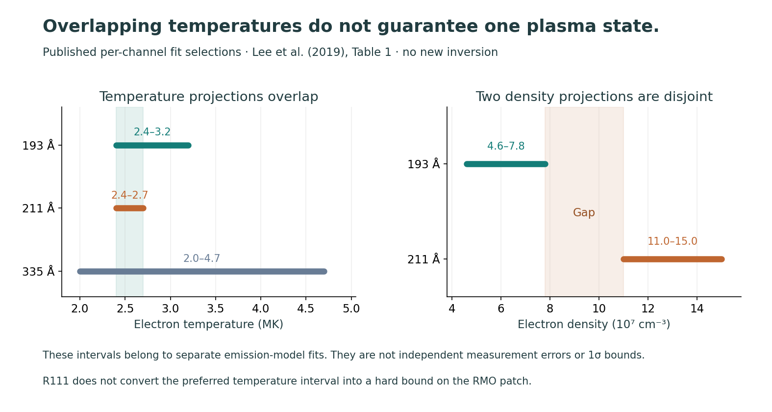
RMO retains 05:38:32.06–05:40:08.06 UTC for the primary 96-s kinematic fit. The source fits the following light-curve intervals:
| Channel | Source fit interval UTC | Overlap with RMO interval | Meaning |
|---|---|---|---|
| 193 Å | 05:39:18–05:41:06 | 50.06 s | Partial overlap; a different fitted interval |
| 211 Å | 05:39:12–05:42:12 | 56.06 s | Partial overlap; a different fitted interval |
| 335 Å | 05:39:15–05:42:15 | 53.06 s | Partial overlap; a different fitted interval |
Time overlap alone does not establish the same plasma state. A fixed aperture contains material heated at different earlier times while the crest moves onward. Nor does a matching nominal image time establish the mask coordinates.
The paper identifies a white box but the inspected source locations do not supply a numeric solar-coordinate centre or a registered pixel mask. We do not place that box on our WCS image by eye. The same-patch and same-state correspondence remain unresolved.
The source temperature is constrained by an emission and ionization model applied to count-rate histories, rather than imposed by the RH temperature-jump formula. This makes it a candidate test of the thermal prediction.
It still depends on a background treatment, ionization history, emitting depth and geometry. It also reuses AIA observations; statistical independence from all RMO data is not established. Independent of one formula does not mean free of assumptions.
R110 supplies total pressure and an equivalent common electron/proton temperature under Tₑ=Tₚ. A NEI electron-temperature estimate becomes a test of that quantity only after the sampled plasma and thermal closure are matched.
The three saved fast examples predict equivalent downstream temperatures of 2.752, 2.863 and 3.127 MK, with fields 1.474, 1.597 and 1.753 G. They are retained model outputs, not new measurements or rerun calculations.
R111 adds no new temperature bound, magnetic prior, uncertainty sweep or fast/slow label. The central slow exclusion remains conditional on R110's inputs. Degenerate and field-reversing candidates keep their previous status. No ordinary or unresolved state is rejected using one source passband interval.
One next observational step: obtain matched 171/193/211/335 Å light curves for one aperture tied to our RMO sector. Define its coordinates, background and front/CME passage first; use a small timed cutout. Keep the 96-s kinematic result separate. This extraction stage should produce observable curves before any new RMO or NEI parameter fit.
Sources: Lee et al. (2019), §3.3, Table 1 and Figs.8–11 (published DOI); Ma et al. (2011), Fig.1 and photometry; unchanged R106–R110 records. New work here: the correspondence decision, time-overlap arithmetic and interval-intersection check. No new solar FITS, photometry, DEM or NEI fit.
13 June 2010 · one central conditional reconstruction
We completed the accepted R109 input set into candidate plasma states. Three checked examples are fast shocks with different fields. A regular slow shock fails the transition equations for these exact inputs.
This is a conditional model result. The radio/temperature transfer, geometry, reference flow and pressure closure remain assumptions. No observational wave family or uncertainty-robust exclusion is claimed.
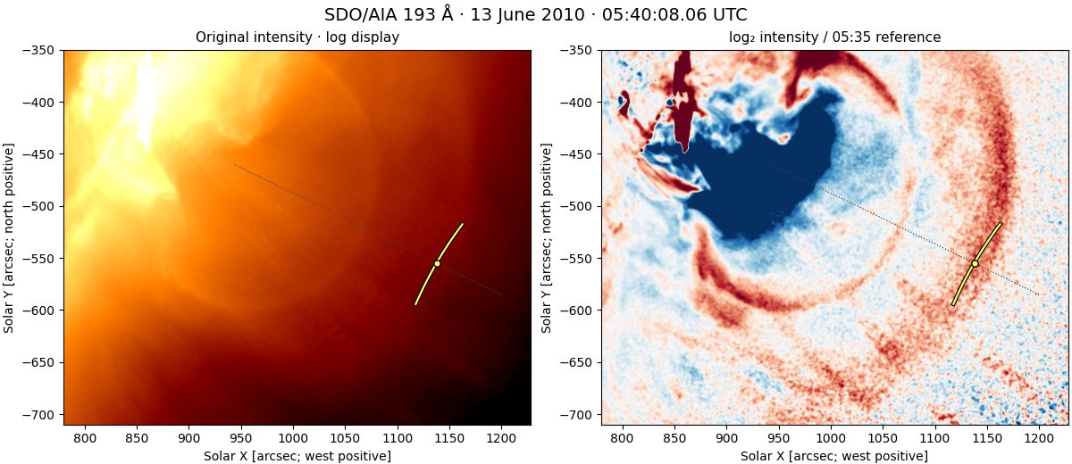
| Parameter | Central value | Origin | Source | Assumption / meaning |
|---|---|---|---|---|
| Crest position and motion | PA116; 707.5 km/s radial mean over 96 s | MEASURED · image-derived | R106–R107, AIA 193 Å | Pattern motion; not plasma velocity. |
| Effective normal speed / inflow | 705.5 km/s | DERIVED + ASSUMED | R109, fixed G0 and reference u₁ₙ=0 | Zero LOS tilt; endpoint normal fixed; no measured flow interval. |
| Radio lanes | 132 and 165 MHz | SOURCE-DERIVED | Ma et al. 2011 §3.2 | Same second harmonic; two sides of one front; transfer to this patch assumed. |
| Density and compression | nₑ₁=5.40×10⁷ cm⁻³; X=1.5625 | DERIVED + ASSUMED | Same radio lanes and plasma-emission relation | X and density share frequencies; they are not independent measurements. |
| Upstream temperature | 1.8 MK | SOURCE-DERIVED + ASSUMED transfer | Ma / Kozarev regional diagnostic; R108 | Adopted for this patch; exact spatial correspondence not established. |
| Pressure and composition | Pure H; Tₑ=Tₚ; γ=5/3; p₁=2.685×10⁻³ Pa | ASSUMED closure + DERIVED pressure | R109 explicit reference | Electron and proton pressures both included; cₛ₁=222.5 km/s. |
| Magnetic strength / angle | Not prescribed | UNKNOWN INPUT → CONDITIONAL OUTPUT | R110 reconstruction | No literature B prior; no source shock-derived B used as independent evidence. |
| Downstream temperature / flow | Reconstructed values in the table | CONDITIONAL OUTPUT | R110 conservation equations | T₂ assumes the same pure-H equal-temperature closure; not independently measured. |
| Uncertainty | Central values only | NOT PROPAGATED | R109 error record retained | Model-to-model differences below are neither ± errors nor confidence intervals. |
Density and compression come from the same radio frequencies. Field strength and angle are left free. The R109 table, with its proposed uncertainty ranges and fuller explanations, is retained unchanged below in QuickLook.
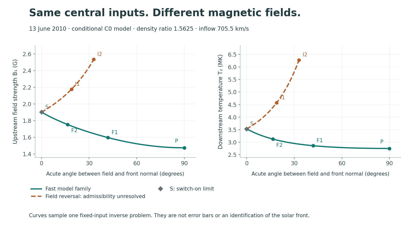
| Model | B₁ (G) | Field–normal angle (°) | T₂ (MK) | Tangential flow change (km/s) | Checked result |
|---|---|---|---|---|---|
| P · perpendicular | 1.474 | 90.00 | 2.752 | 0.0 | Fast supported |
| F1 · oblique | 1.597 | 41.89 | 2.863 | 146.0 | Fast supported |
| F2 · oblique | 1.753 | 16.49 | 3.127 | 268.6 | Fast supported |
| S · switch-on limit | 1.902 | 0.00 | 3.535 | 388.2 | Degenerate; ordinary class unassigned |
| I1 · field reversal | 2.176 | 18.88 | 4.573 | 592.3 | Admissibility unresolved |
| I2 · field reversal | 2.534 | 32.96 | 6.273 | 823.5 | Admissibility unresolved |
B₁ is upstream field strength; the angle is the acute angle between field and front normal. T₂ is the predicted common electron/proton temperature under the stated closure. Every number in this table is a conditional output. Global field polarity and its direction along the front remain free.
All six points pass full conservation and gas-entropy checks. P, F1 and F2 also pass the implemented fast classification. S remains degenerate; I1 and I2 have a tangential field reversal and require additional admissibility assessment. A conserved state is not automatically a selected solar transition.
The plasma enters the front at 705.5 km/s and leaves normally at 451.5 km/s, both measured relative to the front. For P, F1 and F2, the upstream fast speeds are 490.8, 499.4 and 524.9 km/s; their downstream fast speeds are 612.2, 615.5 and 623.0 km/s.
The entering plasma is faster than its local fast speed; the exiting plasma is slower than its local fast speed. The oblique cases also pass the normal Alfvén-speed condition. Field, momentum, total energy and entropy are checked together.
A regular slow shock requires upstream inflow below the normal Alfvén speed. At this particular pressure, inflow and compression, the transition equations would then require a negative squared tangential magnetic field. No real field can satisfy that condition.
The zero-tangential-field exceptions are checked separately: switch-off has the same sign failure; a purely parallel gas jump requires compression 3.081 instead of 1.5625. This exclusion belongs only to the exact central C0 model. It does not rule out a solar slow front under different inputs or a structure containing several waves.
Six representative states and 161 samples of the same central family were checked against the original conservation fluxes. Maximum scaled residual: 1.5 × 10⁻⁷⁹ in 80-digit arithmetic. Independent characteristic-speed calculations agree. A separate Newton solution recovers F1 to 2.23 × 10⁻¹⁶; a frame-conversion check preserves its class.
These small residuals describe the calculation, not observational accuracy. No input-error sweep was run. The existing classifier and earlier scientific results were not changed. Its exact-model input mode applies to each reconstructed pair, not to the accuracy of the observations.
Normalize upstream density and incoming normal speed to 1, and use μ₀=1. Let r=ρ₂/ρ₁=1.5625, b=p₁/(ρ₁U²)=0.0596967, and h=Bₙ²/(μ₀ρ₁U²). U is the incoming speed, Bₙ the normal field, and b the normalized pressure.
N = 4 − r − 5br
S = r + 5 − 2rh(4 − r)
k = √[2N/(rS)]
Bₙ = √h; Bₜ₁ = k(1 − rh); Bₜ₂ = kr(1 − h)
u₂ₙ = 1/r; u₂ₜ = Bₙ(Bₜ₂ − Bₜ₁)
p₂ = b + 1 − 1/r + (Bₜ₁² − Bₜ₂²)/2
These are normalized fields and states for γ=5/3. At h=0.64, the upstream tangential field vanishes: the switch-on limit. The signed formula stays finite there. For a regular slow shock h>1, but N>0 and S<0 would give Bₜ₁²<0. The regular expression has a pole at h=0.861538; plotting stops earlier, at 0.80.
Positive model inflow uses the inward normal, opposite G0’s outward normal. A common tangential boost sets upstream tangential velocity to zero for calculation. It does not supply a measured solar flow. Under the reference outward u₁ₙ=0, all points predict u₂ₙ≈254.0 km/s in the solar frame; the table gives the tangential change across the front.
The next useful measurement: an independent field-direction or downstream thermal constraint for the same patch and interval. It could separate models that fit the present inputs equally well. A temperature or field inferred from the same assumed shock model cannot confirm that model independently.
For a downstream DEM comparison, first establish how its electron-temperature distribution maps to the model’s thermal pressure. T₂ here is not automatically an observed DEM peak. We will first check the correspondence for one candidate constraint; no new robustness campaign starts automatically.
Sources: Ma et al. (2011), Kozarev et al. (2011) and R106–R109 input records. Transition relations: Fitzpatrick; broader intermediate/switch-limit treatment: Takahashi & Yamada (2013). R110 results are new model calculations, not quoted measurements.
13 June 2010 · one proposed reference scenario
We have one consistent set of partial inputs to review. The radio and temperature estimates are assigned to our EUV patch as accepted assumptions. The remaining reference choices are visible below. No MHD calculation has been run.
Already accepted: the radio compression and pre-front temperature represent our selected patch.
Proposed here: both split lanes are the second harmonic from two sides of one front; use the primary 96-s mean as an effective scenario speed; hold G0's endpoint normal fixed; set the upstream reference flow to zero; use fully ionized pure hydrogen with equal electron and proton temperatures and γ=5/3.
These are model choices. Zero flow is not a measurement. The magnetic field and its angle remain unknown; no numerical magnetic prior is imposed.
For one proposed envelope, use 132 ± 5 MHz, 165 ± 15 MHz and 1.8 ± 0.4 MK as simultaneous bounds, allowing all triples. This is a chosen error interpretation, not a claim of 1σ or statistical independence.
The saved R76 radio envelope is X = 1.563 −0.364 / +0.446, approximately 1.20–2.01. The quoted X=1.56±0.10 is not added as another independent constraint.
The image speed's 687–718 km/s method spread remains separate from a full error budget. Transfer errors, flow uncertainty and 3D geometry are not covered by the frequency–temperature box. No robustness claim has yet been tested with these bounds.
| Quantity | Value | Origin | Source | Error / range meaning | Assumption | Use |
|---|---|---|---|---|---|---|
| Patch and fit interval | PA116; 05:38:32.06–05:40:08.06 UTC, 13 June 2010 | MEASURED · image-derived selection | R106–R107 | 96-s fitted interval; not a timing error | The selected brightness crest traces the physical front. | Primary interval retained; no new tracking. |
| Projected radial pattern speed | 707.5 km/s | MEASURED · image-derived diagnostic | R107 primary fit | 687–718 km/s is the saved finite estimator spread, not 1σ or total bounds. | Treat the 96-s mean as an effective scenario speed. | Use the primary fit; keep the 60-s fit separate. |
| Image normal and 3D reference | PA 120.28°; line-of-sight tilt 0° | MEASURED image normal + ASSUMED 3D geometry | R106, G0 | 113–126° is estimator spread; line-of-sight error is unmeasured. | Use the endpoint normal throughout the fit and the G0 tangency outline. | A reference geometry, not measured 3D deprojection. |
| Effective normal pattern speed | 705.5 km/s | DERIVED · measured inputs + assumptions | R107 and G0 | No complete observational uncertainty assigned. | The crest behaves locally as a moving contour; the normal is held fixed. | Multiply radial rate by cos(normal PA − cut PA). |
| Lower / upper radio lane | 132 ± 5 / 165 ± 15 MHz | SOURCE-DERIVED · spectral readout | Ma et al. 2011 §3.2, Fig.7 | For the proposed envelope: 127–137 and 150–180 MHz, all pairs allowed; not 1σ. | Second harmonic; two sides of one front. Patch transfer accepted in R108. | Primitive radio inputs; their error meaning is an explicit scenario choice. |
| Electron density before / behind | 5.40 / 8.44 × 10^7 cm⁻³ | DERIVED · radio diagnosis | Ma §3.2; selected harmonic | Upstream 5.00–5.82; downstream 6.98–10.04, all ×10^7 cm⁻³. | Same radio interpretation and fixed harmonic. | Compute together with X from the same two frequencies. |
| Compression X | 1.5625; proposed envelope 1.199–2.009 | DERIVED · radio diagnosis | Central frequencies; bounds retained from R76 | 1.563 −0.364 / +0.446; hard scenario envelope, not a confidence interval. | Fixed composition across the front. | Do not also impose the quoted X=1.56±0.10 as an independent constraint. |
| Temperature before the front | 1.8 ± 0.4 MK | SOURCE-DERIVED · adopted regional DEM peak | Ma §3.2; Kozarev §3.2 | Proposed envelope 1.4–2.2 MK. Source confidence level and transfer error are unknown. | Transfer to this patch accepted in R108; equal electron/proton temperatures proposed here. | Input temperature, with its origin and transfer visible. |
| Composition and thermal pressure | Fully ionized hydrogen; Te=Tp=T; γ=5/3 | ASSUMED · proposed simple reference | Explicit ideal-plasma closure; same convention used in R104a | Fixed model choice; not a measured abundance or error interval. | Ignore helium, heavier ions and electron mass in this reference. | ρ1=mp ne1; total p1=2 ne1 kB T, using ne in m⁻³. |
| Mass density / total pressure | 9.035e-14 kg/m³ / 2.685e-03 Pa | DERIVED · radio + temperature + closure | R109 stated conversion | ρ1 and p1 inherit the same lower radio lane; p1 also inherits T. | Thermal and composition closure above. | Keep the dependence; do not draw these as independent inputs. |
| Sound speed | 222.5 km/s | DERIVED · total pressure and mass density | cs²=γ p1/ρ1 | 196.3–246.0 km/s under the temperature envelope only. | Fully ionized H with Te=Tp. | This closure does not reproduce the source’s quoted 156 km/s; do not mix conventions. |
| Plasma flow before the front | u1n=0 km/s for the proposed reference | ASSUMED · unmeasured reference | Scenario definition; no independent local spectroscopy in this input set | No observational flow interval available. Zero is not a measurement with zero error. | Static upstream reference only. | w1=Vn−u1n; any future flow change changes the inflow. |
| Magnetic strength and direction | Unknown; no numerical prior imposed | UNKNOWN · quantities to constrain or infer | R108 source audit; Démoulin–Klein reference registry | No independently justified local interval. | Do not insert the source’s shock-derived B or Alfvén speed as independent measurements. | Allow field parameters in a partial-input reconstruction; a full two-state classifier is not ready. |
| Plasma behind the front | Radio-inferred density only; pressure, field and velocity unresolved | PARTIAL · source-derived density; remaining state unknown | Same radio lanes | No independent downstream thermal/magnetic bounds. | Candidate states must satisfy the chosen physical model. | Do not manufacture the missing state or assign an MHD family. |
In the proposed hydrogen model, electrons and protons both exert pressure. With equal temperatures, the total pressure is p₁ = 2 nₑ₁ kBT and the mass density is ρ₁ ≈ mpnₑ₁. The sound speed follows from cs1² = γp₁/ρ₁.
At 1.8 MK this gives 222.5 km/s. The temperature envelope 1.4–2.2 MK gives 196.3–246.0 km/s under this same closure. Here kB is Boltzmann's constant and mp is the proton mass; density is converted to m⁻³ in the pressure formula.
The source's quoted 156 km/s is not an independent measured speed to insert alongside this temperature and pressure convention. The simple hydrogen composition and equal temperatures are assumptions, not a complete description of solar abundances.
With second-harmonic plasma emission, nₑ₁ = [fL/(2K)]² and nₑ₂ = [fU/(2K)]², where K=8980 Hz for density in cm⁻³. Thus X=nₑ₂/nₑ₁=(fU/fL)². One pair of frequencies supplies all three numbers.
Keep this dependence in any later uncertainty calculation. Do not vary density, compression, pressure and sound speed independently when they come from shared inputs.
The crest crosses a fixed radial cut. For a local moving contour, Vn,POS = (dr/dt) cos(ψ−PAcut). The normal angle ψ is 120.2765° and the cut angle is 116°, measured clockwise from north. Holding that normal fixed gives 705.5 km/s from the retained 707.5 km/s radial mean.
G0 assumes zero line-of-sight tilt. This is an effective pattern speed under the stated geometry, not an instantaneous or independently deprojected physical speed. The separate last-minute fit would give 575.1 km/s with the same conversion; it does not replace the primary fit.
The speed of plasma entering the front is w₁=Vₙ−u₁ₙ. With the proposed reference u₁ₙ=0, w₁≈705.5 km/s and acoustic M₁≈3.17. An actual upstream flow would change these values.
Missing B does not make the event unusable. A partial-input reconstruction can seek candidate field parameters and missing states. Its inferred field is a conditional result, not an independent confirmation of the same model. Typical literature values are available as context; they do not automatically define local bounds.
One next step: after review of this reference scenario, perform one central reconstruction and check the candidate states. Keep all adopted assumptions beside the answer. No uncertainty sweep follows automatically.
Sources: Ma et al. (2011), Kozarev et al. (2011), and the saved R76/R106–R108 records. Démoulin & Klein (2000) supplies typical environments, not a local magnetic error interval. No observed MHD family is identified here.
13 June 2010 · checking the origin of our inputs
For this scenario, we assign the published radio compression and pre-front temperature to our selected EUV patch. This transfer is an adopted assumption. The papers support a link to the event, but do not independently establish the same local plasma sample.
| Input | What we have | What we must assume |
|---|---|---|
| Our EUV crest | Image-derived position and interval-mean speed at PA116 | How this bright ridge traces a physical front |
| Radio compression | Published X = 1.56 ± 0.10 around 05:40 | The radio source is this EUV segment; the lanes sample opposite sides of one front |
| Pre-front temperature | Published/adopted T = 1.8 ± 0.4 MK from extended DEM regions | That earlier regional temperature represents our later local plasma ahead of the front |
Published estimates are SOURCE-DERIVED. The transfer to our local patch is an ADOPTED ASSUMPTION for this scenario. Quoted ± values are not automatically 1σ or simultaneous hard bounds.
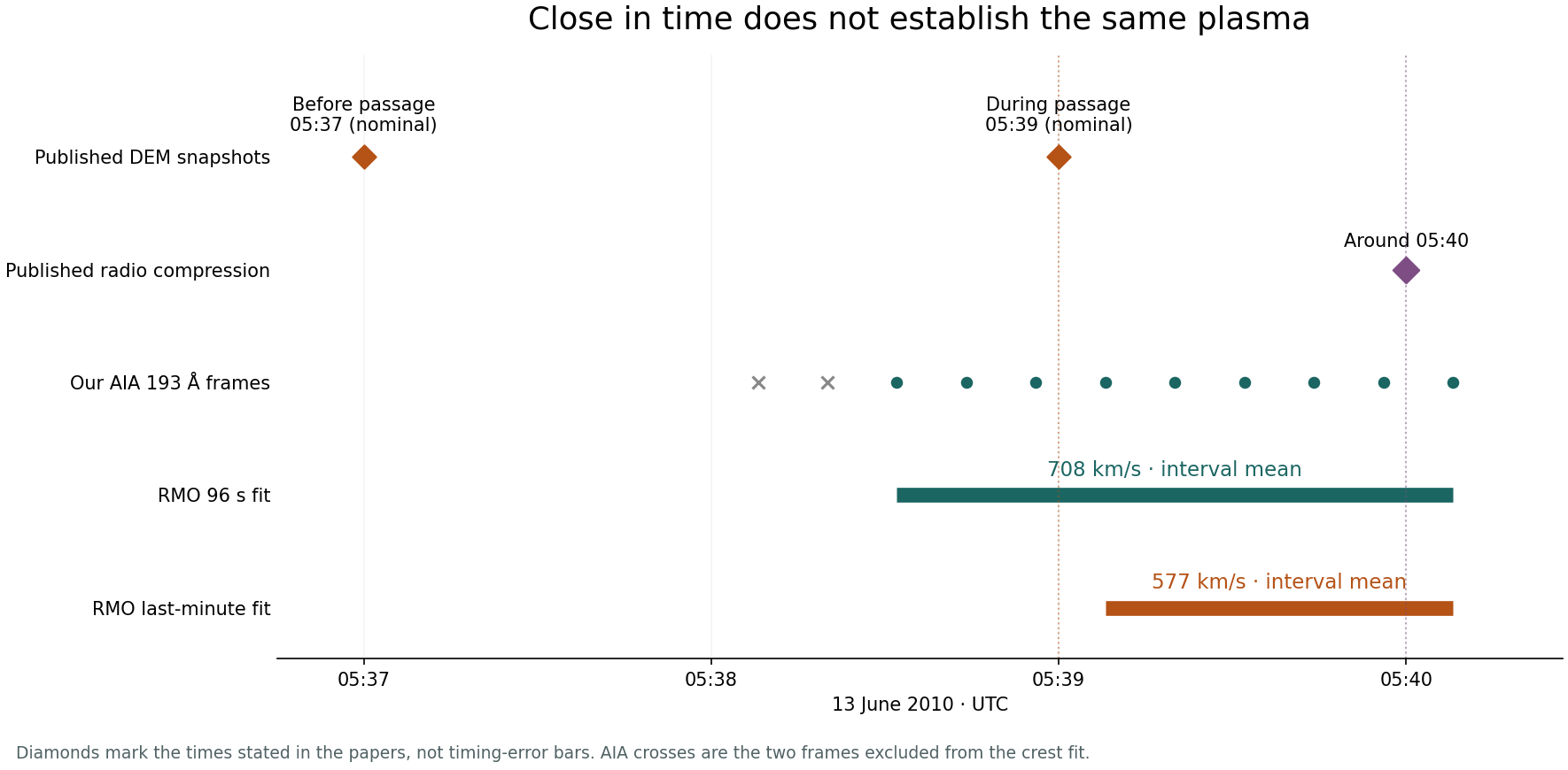
The left image in each pair shows intensity. The right shows its ratio to the reference image. Yellow marks our measured EUV crest; it is not a DEM mask or a located radio source.
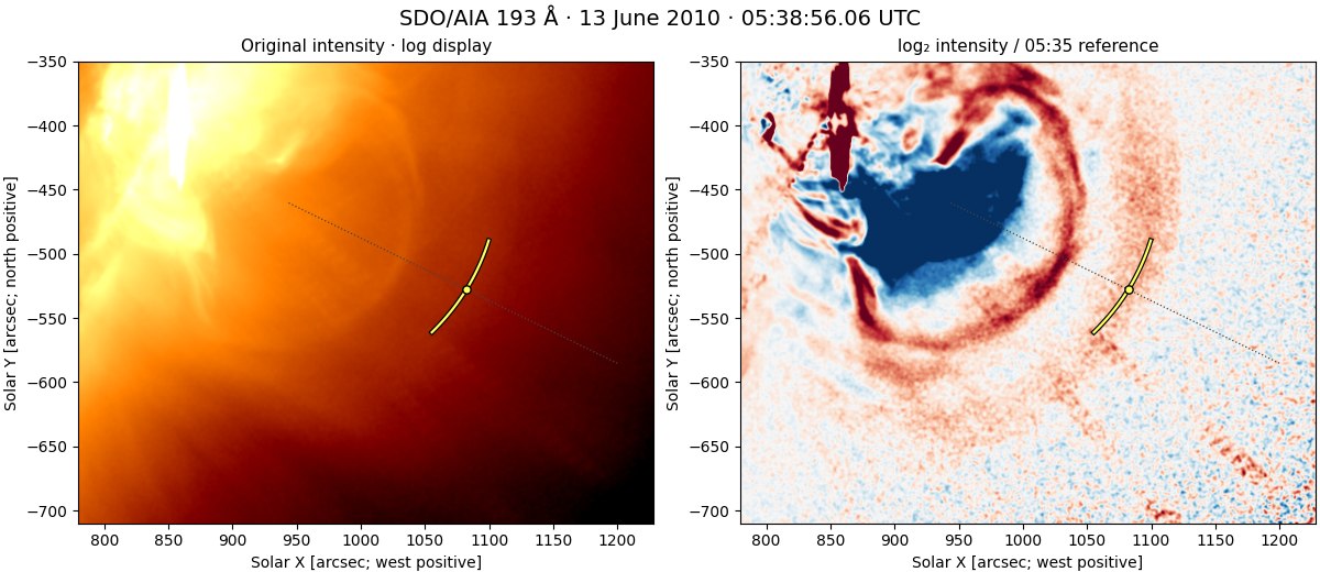
About 4 s before the nominal 05:39 DEM time. This temporal proximity alone does not register the published DEM regions onto our patch.
End of our measured sequence, near the published radio epoch. Both views use the saved R107 display and crest; no new tracking was performed.
Ma et al. (2011), §§2, 3.2–3.3 use San Vito radio spectra and quote the split near 05:40. A spectrum shows frequency versus time; it does not give the emitting patch's sky coordinates. Their radio heights depend on a density model. The temperature is adopted from Kozarev's R2/R3 DEM peak, with a stated regional difference.
Kozarev et al. (2011), §3.2 and Fig.3 compare six-channel DEMs in extended regions at nominal 05:37 and 05:39. R2 and R3 provide results. R1 and the upstream comparison R4 do not provide statistically significant DEM results. Exact masks registered to our FITS are not supplied by this comparison. We do not claim that the masks overlap, or do not overlap, our fitted crest.
Their regional density-change estimates, about 1.18 and 1.12, depend on a simplified emission model. They are not an additional direct measurement of the same local X to average with 1.56.
Radio frequency depends on electron density. If the two lanes are the same harmonic emitted on opposite sides of one local front, their ratio gives
X = (fhigh / flow)2.
Here X is the electron-density ratio behind versus ahead of the front. With a consistent composition, it also represents the mass-density ratio. The formula does not locate the radio source. We still need an assumption that connects the emitting plasma to our EUV patch.
DEM describes the amount of emitting material at different temperatures along the line of sight. Its peak is not automatically the temperature just ahead of one thin front. For a simple uniform column, EM ≈ ne2L: density and emitting depth both matter. Background emission adds another dependence.
| Quantity | Origin | Permitted role at this stage |
|---|---|---|
| R106–R107 geometry and motion | MEASURED · image-derived diagnostic estimates | Saved local image inputs, with their projection and interval limits |
| Radio X and density | SOURCE-DERIVED · shared frequency information | Conditional inputs; shared dependence and error meaning must be retained |
| DEM-peak temperature | SOURCE-DERIVED · regional estimate | Conditional environment-temperature input |
| Radio/temperature transfer to this patch | ASSUMED · adopted for this scenario | Must be stated with every resulting scenario |
| Published B, Alfvén speed and post-front temperature | SOURCE-DERIVED · model outputs | Later model comparisons; not independent validation inputs |
| Upstream flow and independent field constraints | UNKNOWN | Need explicit, physically justified limits before a model run |
The event remains useful. RMO can show what follows under stated assumptions and which missing observation would change the conclusion. This step does not identify a fast or slow shock.
One next step: complete the conditional input table, retaining the adopted transfers and specifying flow, field, geometry and uncertainty meanings. A model run follows only after those choices are settled.
Solar observations · 13 June 2010 · one measured patch
The same outer EUV ridge is now tracked through a short AIA sequence. Its mean projected radial speed depends on the time interval. The result is an image-derived motion estimate; it does not yet identify an MHD family.
| UTC interval | Frames | Mean projected speed | Finite method spread |
|---|---|---|---|
| 05:38:32–05:40:08 · 96 s | 9 | ≈708 km/s | 687–718 km/s |
| 05:39:08–05:40:08 · last 60 s | 6 | ≈577 km/s | 542–608 km/s |
These ranges compare 18 ways of locating the crest. They are not ±1σ, complete uncertainty bounds or two errors on the same mean. Neither fit gives an instantaneous speed at 05:40. A changing brightness profile can contribute to the interval dependence.
SDO/AIA 193 Å · 13 June 2010. Yellow: fitted outer ridge; dot: its position at PA 116°. The first two frames have no fitted outer crest.

2010-06-13T05:38:08.07Z · no fitted outer crest
Actual observations are about 12 s apart; playback speed is only a viewing choice. Left: exposure-normalized intensity with a fixed log stretch. Right: log₂ intensity ratio to 05:35:08.07 UTC. This is not a density or compression map.
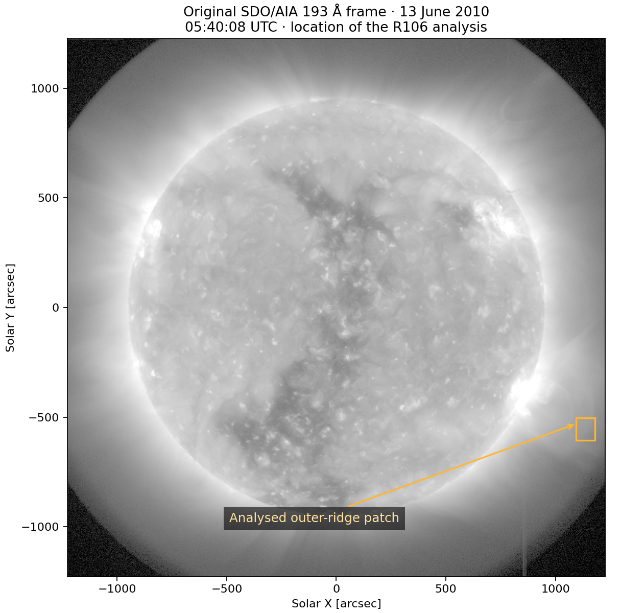
Original solar context retained from R106; the kinematic measurement follows the same outer ridge.
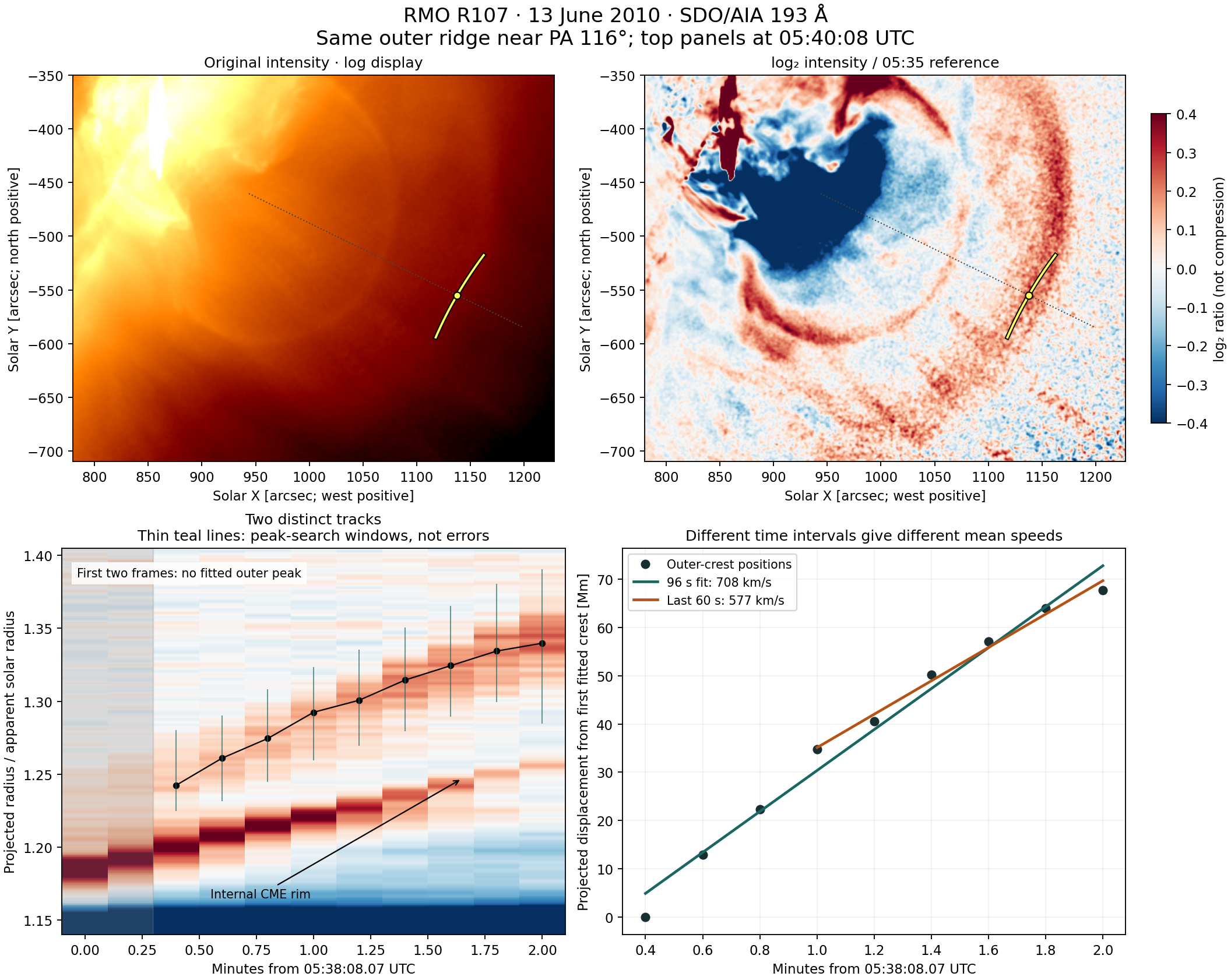
| Input or result | Origin | Meaning / limitation |
|---|---|---|
| AIA 193 Å intensity; 12 FITS | MEASURED · SDO/AIA archive via VSO | 11 science frames plus reference; QUALITY=0; all selected frames received. |
| T_OBS, exposure, WCS, observer distance | Archive observation metadata and SOURCE-DERIVED instrumental geometry | Actual 11.98–12.03 s cadence. Header WCS alignment, not separately certified image registration. |
| PA=116° patch | SOURCE-DERIVED selection from Ma et al.; image-derived fitted positions | Local ±2° central fit; final point matches R106. |
| Outer-crest position and mean speed | MEASURED · diagnostic estimates from original FITS | Projected radial pattern motion. The emission ridge / physical front association remains ASSUMED. |
| Line-of-sight geometry | ASSUMED scenario G0 from R106; actual tilt UNKNOWN | No automatic speed deprojection or normal-speed conversion. |
| Upstream plasma flow, B direction, θBn | UNKNOWN | No zero-flow substitution; no plasma-frame speed or MHD classification. |
| Density/compression and temperature | Not inputs to this fit | Published radio/DEM constraints remain in R105; matching to this patch is still required. |
Each Level 1 frame is exposure-normalized, smoothed with σ=1.5 native pixels and sampled on the same WCS grid. The first two science frames remain visible but are excluded from the speed fit because the outer local peak is insufficiently separated. Per-frame windows isolate the outer crest independently of any expected speed. They were chosen before fitting and are saved with the result.
Local quadratic radius-versus-PA fits provide the PA116 crest position. The central method uses log-ratio, radial smoothing σ=4 samples and a ±2° window. Two observables, three radial smoothings and three local windows give 18 related method variants. No fitted peak hits a window boundary; detector coverage and inactive ratio floor were checked. A linear radius-versus-time fit uses actual mid-exposure times and ≈736.699 km per arcsec.
The 96 s fit has 4.09 arcsec RMS residual; the last-minute fit has 1.78 arcsec. Residuals are not astrometric errors. Unknown registration/calibration effects, line-of-sight geometry and changing temperature/ionization/emission profiles remain outside a complete error budget. No extra derotation, PSF correction, temporal interpolation or full calibration certification is claimed. The reference is not certified as globally pre-event.
Ma et al. (2011), §3.1.2 provide an approximate 600 km/s linear scale and a polynomial speed evolution around 600–550 km/s for this event. The last-minute estimate is close to that scale; the full 96 s mean is higher. Different intervals and crest definitions prevent a claim of complete numerical reproduction. The literature speed was not an input to this tracking.
R107 supports a reproducible kinematic input from real observations, with an explicit feature and interval. It does not establish plasma-frame speed, shock type or magnetic field. No full RMO run or generic robustness test was performed.
Next proposed step: check whether the published radio compression and temperature can be assigned to the same time and EUV patch before combining them into one conditional RMO input set.
13 June 2010 · one local geometry step
Yes, as a labelled geometry scenario. The candidate normal to the observed excess-emission ridge is about 120° clockwise from solar north. Eighteen estimator choices give about 113–126°. This is method spread, not a confidence interval or a certified physical bound.
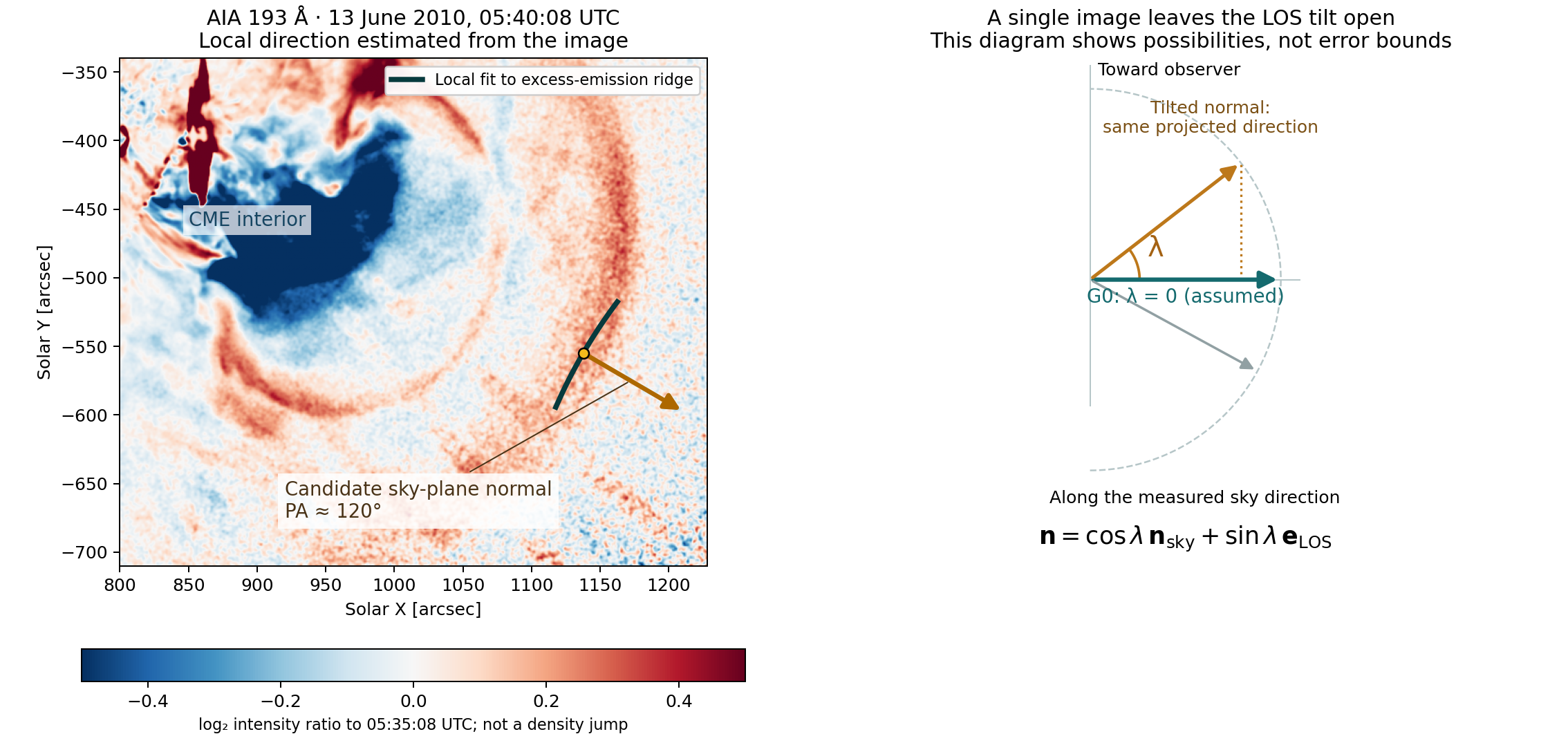
| Quantity | Value / status | Origin and meaning |
|---|---|---|
| Sky-plane ridge-normal direction | About 120°; methods 113–126° | MEASURED diagnostic estimate from the two AIA FITS; identifying this emission ridge with a physical front is an assumption. |
| Line-of-sight tilt λ | G0: λ = 0 | ASSUMED: treat the visible ridge as a tangency outline of a thin, smooth front. Its actual tilt range remains unknown. |
| Local 3D normal in G0 | n ≈ (0.864, −0.504, 0) | ASSUMED full geometry, informed by the measured projection. X west, Y north, Z toward the observer. |
| Field-to-normal angle θBn | Unknown | The image-normal estimate does not determine the magnetic-field direction. |
This is one local normal, not a normal for the whole dome. The family n(λ) = cos(λ) nsky + sin(λ) eLOS remains available for later conditional analysis. No numerical tilt interval has been assigned from guesswork. A speed deprojection is not inferred from this expression.
The two original Level 1 images were exposure-normalized, smoothed by σ=1.5 native pixels and sampled on a common WCS grid. No extra registration, derotation, PSF correction or calibration certification was performed. A local quadratic r(PA) fit uses the outer peak in 1.285–1.390 apparent solar radii near PA=116°. The central estimator uses the log intensity ratio, a ±2° fitting window and radial smoothing σ=4 samples. Comparison covers two observables, three smoothings and three fitting windows. All fitted peaks remain inside the search window and detector coverage.
The fit residual and estimator spread are not observational confidence intervals. Line-of-sight integration, feature definition, residual registration, actual 3D shape and matching to radio/DEM diagnostics remain open. The 05:35 reference is not certified as globally pre-event. No new FITS download, front-speed fit, RMO run, uncertainty sweep or solar family classification was made in R106.
Our event list includes candidates, literature comparisons and control cases; it does not supply a positive RMO label in advance. R105 below remains the earlier input-inventory snapshot. R106 updates its geometry item only.
One next step: measure the speed of the same outer ridge using a short AIA 193 Å sequence. It has not been measured from these two frames here.
Selection references: Ma et al. (2011), §3.1.2 and Figs. 1, 3–4; Kozarev et al. (2011). The ≈120° estimate is a new R106 image-derived quantity, not a number copied from those papers.
13 June 2010 · observational input review
Только таблица для согласования. Расчёт RMO и sweep не выполнены. Выбран внешний EUV-купол около 05:40 UT. Получены два AIA 193 Å FITS; новая скорость и нормаль пока не измерены.
MEASURED — собственное считывание данных/метаданных; SOURCE_DERIVED — опубликованная диагностика или модель; ASSUMED — предположение; UNKNOWN — значение не задано. Неуточнённые ± не названы 1σ. Происхождение каждой величины сохраняется вместе с её физическим смыслом.
| Параметр | Значение | Происхождение | Источник | Ошибка / диапазон | Пригодность для RMO | Чего не хватает |
|---|---|---|---|---|---|---|
| Данные и время | SDO/AIA 193 Å; два FITS: 05:35:08.07 и 05:40:08.06 UTC | MEASURED · метаданные файлов | Заголовки двух полученных Level 1 FITS; T_OBS, EXPTIME, QUALITY | Экспозиции 2.900862 и 2.900866 с. T_OBS — середина экспозиции, DATE-OBS — её начало; это не ошибка времени. | 4096 × 4096; 0.600758″/пиксель; QUALITY=0. WCS доступна. Калибровка и совмещение ещё не проверены. | В каталоге 40 записей с шагом 12 с; скачаны только два кадра. Они не образуют временной ряд для надёжной новой скорости. |
| Участок фронта | Внешний EUV-купол перед CME около 05:40 UT; опубликованные радиальные направления 115°, 116°, 117° от севера по часовой стрелке | SOURCE_DERIVED · выбор по изображениям статьи | Ma et al. (2011), §3.1.2, Figs. 1, 3 | Шаг между направлениями не является погрешностью нормали. | Обоснованный участок для первого наблюдательного примера. Внешний фронт и границу CME нужно прослеживать раздельно. | Точная общая область/момент EUV, радио и DEM ещё не установлены. Направление радиального разреза не равно измеренной нормали. |
| Геометрия / нормаль n | 3D-нормаль неизвестна; новая 2D-нормаль не измерена | UNKNOWN | Ma et al. (2011), §2, Figs. 1, 5; WCS новых FITS | Численная ошибка нормали пока не задана. | Событие у лимба облегчает наблюдение внешнего купола, но не устраняет проекцию. | Локальная касательная к выбранному фронту, её ошибка и ограничение наклона по лучу зрения. STEREO-контекст сам по себе не даёт восстановленной 3D-нормали. |
| Скорость фронта | Около 600 → 550 км/с в опубликованной эволюции | SOURCE_DERIVED · траектория яркостного максимума | Ma et al. (2011), §3.1.2, Figs. 3–4 | Это изменение во времени, НЕ 575 ± 25 км/с и НЕ измеренная ошибка в 05:40. | Ориентир для будущей независимой траектории. Сейчас не новая измеренная нормальная скорость RMO. | Скорость того же участка в выбранный момент, ошибка положения/подгонки, проекционная поправка; определение максимума яркости либо переднего края. |
| Скорость плазмы перед фронтом u₁·n | Неизвестна | UNKNOWN | В рассмотренных материалах нет независимого измерения для выбранного участка | Ни центральное значение, ни допустимый интервал не приняты. | Для скорости в системе фронта нужна разность между движением фронта и плазмы. | Спектроскопия или явно обоснованная модель потока. u₁=0 нельзя молча считать измерением. |
| Две радио-полосы | fL = 132 ± 5 МГц; fU = 165 ± 15 МГц около 05:40 UT | SOURCE_DERIVED · опубликованное считывание спектра | Ma et al. (2011), §3.2, Fig. 7 | Цитированные ±; статистический уровень и совместная зависимость не установлены в доступном описании. | Более близкие к наблюдению величины, чем выведенные из них X, n₁, B. Спектр здесь не измерен заново. | Смысл ширины полос/ошибки считывания, их совместность; идентификация гармоники и связь радиоисточника с EUV-участком. |
| Сжатие X = ρ₂/ρ₁ | В статье X = 1.56 ± 0.10 | SOURCE_DERIVED · радио-диагностика | Ma et al. (2011), §3.2, Eq. (3) | Опубликованная ±0.10; её согласование с ошибками обеих частот остаётся открытым (сохранённый аудит R76). | Условно при интерпретации расщепления как излучения до/после одного перехода и неизменном составе. X=(fU/fL)². | Нельзя одновременно объявить ±0.10 и обе частотные ± независимыми жёсткими границами. Нужен согласованный выбор модели ошибок. |
| Плотность до фронта nₑ₁ | Около 6 × 10⁷ см⁻³ | SOURCE_DERIVED · радио-плазменная частота | Ma et al. (2011), §3.2, около 05:40 UT | Приближённая опубликованная оценка; независимая полная погрешность не дана. | Зависит от отождествления полосы/гармоники и её пространственной связи с фронтом. Коррелирует с X через радио-частоты. | Для ρ нужен состав. Один канал AIA не даёт независимые nₑ и глубину излучающего слоя. Яркость EUV не подставляется вместо плотности. |
| Температура до фронта T₁ | 1.8 ± 0.4 МК | SOURCE_DERIVED · DEM соседних областей | Ma et al. (2011), §3.2, со ссылкой на regions 2–3 Kozarev et al. (2011) | Цитированная ширина; Ma прямо отмечают некоторое отличие областей. Не объявлена здесь 1σ. | Полезное ограничение окружения. Не новая DEM-оценка нашего точно выбранного участка. | Пространственно-временное сопоставление DEM с фронтом; вклад фоновой плазмы, многотемпературность и ошибка переноса между областями. |
| Звуковая скорость cₛ₁ / давление p₁ | В статье cₛ₁ = 156 ± 30 км/с; p₁ независимо не измерено | SOURCE_DERIVED · термодинамическое преобразование | Ma et al. (2011), §3.2 | Производная от температуры и выбранной массы частицы/состава; не независимый вход вместе с T₁. | Для RMO нужно согласованно связать ρ, полное давление, T и γ. Число из статьи не принимается автоматически. | Состав, электронная/ионная температуры или их замыкание; согласованная модель ошибки p₁/ρ₁. |
| Поле B₁ / альфвеновская скорость cA₁ | В статье B ≈ 1.3 G; cA ≈ 450 ± 30 км/с | SOURCE_DERIVED · МОДЕЛЬ СКАЧКА | Ma et al. (2011), §3.2, Eq. (4) и последующий текст | Модельная оценка с зависимостью от X, скорости и магнитной геометрии; авторы допускают большую фактическую ошибку. | Сохранено как результат статьи для сопоставления. Не независимое измерение B и не подтверждение типа в новом RMO-тесте. | Независимое ограничение поля и направления либо отдельно согласованные сценарии. Это полная cA, а не cA,n = cA |cos θBn|. |
| Угол θBn между полем и нормалью | Не измерен; 90° используется в перпендикулярной модельной реконструкции | ASSUMED · предположение источника; не принято для нового прогона | Ma et al. (2011), §3.2–3.3 | Измеренного интервала нет. Дуга EUV не задаёт направление магнитного поля. | Перпендикулярный сценарий можно рассмотреть только с явной меткой предположения. | Поле и 3D-нормаль должны быть ограничены совместно. Нельзя заменять θBn геометрическим углом разреза. |
| Температура после фронта T₂ | В статье 2.8 ± 0.6 МК | SOURCE_DERIVED · ПРЕДСКАЗАНИЕ МОДЕЛИ СКАЧКА | Ma et al. (2011), §3.3, Eqs. (5)–(7) | Наследует входы и замыкание реконструкции. | Сохранено как модельный результат. Не независимая измеренная T₂ для проверки той же реконструкции. | Независимая тепловая диагностика и/или отложенные эмиссионные наблюдаемые того же участка. |
| Остальные компоненты двух состояний | u₂, касательные скорости, компоненты B₁/B₂ и независимое p₂ не заданы | UNKNOWN | Текущая таблица источников | Интервалы пока не приняты. | Частично ограниченная диагностика возможна после задания явной области допустимых состояний; полный точечный вход пока отсутствует. | Нельзя заполнять неизвестные модельными выходами и затем называть результат независимой классификацией события. |
B≈1.3 G и T₂≈2.8 МК — выходы опубликованной модели скачка. Они не подставлены как независимые измерения для подтверждения этой же интерпретации.
Главные пробелы: один и тот же EUV/radio/DEM-участок, 3D-нормаль, скорость плазмы, независимое поле и направление, согласованная трактовка ошибок радио-частот. Одобрение таблицы само по себе не задаёт полный набор состояний.
Сохранённые проверки достаточны для начала работы с данными в своей области применимости. Новый общий robustness-test не требуется до просмотра входов; отдельный новый тест должен отвечать конкретной непроверенной постановке или выводу статьи.
Остановка для физического просмотра. Здесь нет новой классификации солнечного события. 40 записей каталога — не скачанная последовательность: получены два кадра, всего 24.41 MB, с T_OBS 05:35:08.07 и 05:40:08.06 UTC. Первый не сертифицирован как полностью предсобытийный. Дальнейшее получение данных отложено.
Источники: Ma et al. (2011), §§3.1.2–3.3, Figs. 1, 3–4, 7; Démoulin & Klein (2000), Table 1. Температурное ограничение Kozarev приведено по Ma §3.2. Радио-интервал перенесён из сохранённого R76 без нового расчёта.
Real EUV event · 13 February 2009
The 3D correction lowers the surface pattern speed from about 260 to 207 km/s, a reduction of about 20%.
T. Podladchikova et al. (2019), Tables 4–5. RMO reproduces the published comparison for the same selected front patch. Its MHD type is not determined by these measurements alone.
Checked model examples · RMO
RMO identified a fast shock, a slow shock, a contact and a rotational discontinuity from the supplied states and front speeds.
No type label was supplied to the diagnostic. Separate calculations of conservation laws and characteristic speeds agreed. These are four known model cases with exact inputs.
13 June 2010 context · Ma et al. (2011) / Kozarev et al. (2011) · Conditional RMO model
In this model, the fast shock remains supported across the adopted input ranges and a field-to-normal angle of 83.3°–90°.
We now vary the speed, thermal and compression constraints together with the field direction. The magnetic strength and the plasma states behind the front are calculated consistently from the conservation laws.
In words: the result does not require perfectly exact inputs or a perfectly perpendicular field. The angle range is a model test, not a measured uncertainty of the solar event.

Read the plot: the entire blue range is above one and the entire green range below one. Conservation, compression and entropy checks also pass. These bars enclose the calculated possibilities; they are not probabilities.
Save vector figure · PDF · Save explanation and checks · Save inputs and results · JSON
Click a Save link to choose a file name and folder when supported. Otherwise, your browser uses its download settings.
Download PDF normally · Download report normally · Download JSON normally
In Windows Chrome press Ctrl+J to find ordinary downloads. To select a folder every time, enable “Ask where to save each file before downloading” in Chrome Settings → Downloads.
The angle is between the upstream magnetic field and the normal, the direction perpendicular to the front surface. At 90° the magnetic field lies along the surface. At 83.3° it tilts away from that configuration by 6.7°.
Every adopted combination of scalar inputs contains this checked angle range. It is a sufficient tested range. We have not shown that the type changes outside it, and we have not measured this angle on the Sun.
| Input | Adopted range or condition |
|---|---|
| Compression | About 1.1988–2.0088, from the saved radio-based constraint |
| Normal inflow | 495.77–667.03 km/s, using the saved speed envelope and an upstream plasma at rest |
| Upstream sound speed | 126–186 km/s, from the saved thermal range |
| Field angle | 83.3°–90°, a common contained model range |
| Model | One planar ideal-MHD front, gamma = 5/3, same source and composition assumptions |
The adopted scalar limits are treated as simultaneous outer bounds. A measured covariance or confidence probability has not been supplied. Downstream field, pressure and velocity are linked by the equations and are not varied independently.
A fixed interval covering checks the entire selected model domain. Seventeen independent full-flux reconstructions and characteristic-speed calculations agree with the unchanged local diagnostic. The finite controls check the implementation; the continuous-domain argument supports the range statement.
For the actual solar front: the local field angle, plasma motion and association of radio, EUV and thermal measurements still need constraints. A compatible model is not yet an independent identification of the observed wave. Open the published evidence and remaining measurements.
Sources: Ma et al. (2011), Kozarev et al. (2011); MHD jump conditions and classes.
# RMO93 — input ranges and field tilt checked together

**Result in one sentence:** The fast-shock interpretation of this model survives the adopted input ranges together with a field-to-normal angle from 83.3° to 90°.

This is a robustness result for a constructed ideal-MHD model motivated by the 13 June 2010 event. It is not an independent determination of the observed EUV-front type. It joins the earlier perpendicular scalar-range check (RMO89) and the central-state field-tilt check (RMO92).

## What changed, in ordinary words

Previously we checked input ranges with an exactly perpendicular field, and separately tilted the field in one central model. We now allow both changes together. We change the input constraints, then solve for magnetic strength, pressure and velocity consistently on both sides of the front. We do not add unrelated noise to the calculated downstream quantities.

For all adopted scalar input ranges there is a common model angle interval from 83.3° to 90°. The plasma still enters faster than the fast-mode speed and leaves slower than it, with compression, magnetic amplification and entropy increase. Full conservation and the downstream super-Alfvénic normal-flow condition also hold. These combined checks support the fast-shock class for this constructed local family.

The angle is measured between the upstream magnetic field and the front normal. At 90° the field lies in the front surface. An angle of 83.3° is a departure of 6.7° from that case. This chosen tested range is not an observational uncertainty, not a maximum allowable tilt, and not a claim that the wave changes type at 83.3°.

## Inputs, provenance and units

| Quantity | Adopted range | Meaning |
|---|---|---|
| Density compression r | 22500/18769 to 32400/16129 (about 1.1988–2.0088) | Previously saved radio-based range under its lane-identification assumptions |
| Normal inflow U1 | 495.77–667.03 km/s | Previously saved speed envelope, treated as normal shock speed with upstream plasma at rest |
| Upstream sound speed c1 | 126–186 km/s | Previously saved thermal range with the same composition assumptions |
| gamma | 5/3 | Fixed model choice |
| Normal-field parameter h | 0–0.01 | Chosen model extension, not a measured magnetic angle |
| Common field-to-normal angle | 83.3°–90° | Contained in the certified domain for every adopted r and thermal ratio |

The source record and its SHA256 are saved in the JSON. The scalar bounds are treated as simultaneous hard outer limits. We do not assign a confidence level, assume a measured covariance, or claim that all combinations occurred on the Sun. Unknown association of the radio, EUV and thermal patches remains explicit.

## Algebraic reconstruction

In units rho1 = U1 = mu0 = 1, let b = c1²/(gamma U1²) and h = Bn²/(mu0 rho1 U1²). The enclosing b range is [1944000/90801841, 207576000/2457878929]. This ratio encloses all combinations in the adopted U1 and c1 ranges; it is not a new independent measurement.

For gamma = 5/3 define

```
M = 4-r-5br
d = 1-rh
W = r+5-2rh(4-r)
q = r(1-h)/d
A = 2M d²/(rW)
N = b r²[5r+1-2h(4r-1)] + (r-1)³
p2 = N/(rW)
```

Then rho2=r, un2=1/r, Bn1=Bn2=sqrt(h), Bt1=sqrt(A), Bt2=q sqrt(A), and ut2=sqrt(hA)(q-1). The upstream tangential velocity and second tangential components are zero. The reconstruction follows one continuous coplanar branch; the physical diagnostic itself receives no input family label.

Mass and normal-field continuity are built into these expressions. Tangential momentum determines ut2. Induction, normal momentum and total energy are checked as exact polynomial identities after clearing the positive denominators. These simplified expressions agree exactly with the earlier RMO92 algebra at the independent controls.

## Entropy and characteristic conditions throughout the domain

All 128 fixed cells of an 8 × 4 × 4 partition in (r,b,h) are checked by outward-rounded 50-digit interval arithmetic. This is a covering of a continuous domain, not a fraction of random trials. Positive M, d, W, A and p2 hold, with r>1 and q>1.

The entropy argument avoids treating correlated pressure and compression as unrelated intervals. Exact algebra gives

```
dp2/dh = 2 M (r-1)³/W² > 0
p2(0)(4-r) - b(4r-1) = A(0)(r-1)³/2 > 0.
```

Thus the entropy increase is at least the gas-Hugoniot value at the smallest compression. Its positive derivative in r has numerator 20(r-1)². The resulting lower enclosure for entropy change divided by cv is 0.0014871475049217420582322361124611737540351547578899. Energy conservation remains a separate requirement; entropy constancy is not substituted for it.

For the upstream state, the magnetosonic matrix trace is below un1²=1, which places its largest eigenvalue below the squared inflow speed. For the downstream state, its magnetosonic characteristic polynomial at un2² has a strictly negative value, placing the normal flow between the slow and fast speeds. The downstream normal flow exceeds the normal Alfvén speed because 1-rh>0. All signs are checked over every cell. Quantitative Mach bounds use the stable magnetosonic discriminant. Downstream scaling is simplified algebraically before interval evaluation to avoid repeated artificial dependence on r.

The resulting outer enclosures over the full (r,b,h) domain are:

| Quantity | Outward numerical enclosure |
|---|---|
| Upstream fast Mach | 1.1199803342954961148975377192067523747727135650837 to 1.9843537938201525349807875020541435216014529586962 |
| Downstream fast Mach | 0.58242253303646670785744819921850002723746603127782 to 0.94331002409022115466976821740450554779053545434143 |

The figure displays rounded labels; the full decimal enclosures are in JSON. These bars are mathematical bounds, not probability distributions. They also enclose the common 83.3°–90° subdomain.

## Why the common angle range is valid

A decreases with r, b and h in the certified domain. For r, the derivative of M is negative, d is nonincreasing, and W+r dW/dr is positive. For b, dA/db = -10d²/W. For h, the derivative sign follows from W-(4-r)d = 2r+1-rh(4-r)>0. These required signs are checked on the domain.

Consequently the largest terminal angle at h=0.01 occurs at the smallest r and b. Its outward interval is 83.231591939875001708461977142396395250102557688468 to 83.231591939875001708461977142396395250102557688573. For each r,b, the angle varies continuously and strictly from 90° down to a terminal angle no larger than that value. Every pair therefore contains the conservatively stated interval 83.3°–90°.

Arctangent bounds use an alternating power series with an explicit remainder. Pi is enclosed with Machin's identity, using the same outward arithmetic. The larger certified h domain contains angles down to about 75.87° for some inputs; this is not a common angle interval for all inputs, so it is not used as the headline result.

## Independent checks

Seventeen model controls comprise the 16 combinations of the endpoint r, U1, c1 and h values, plus one interior state. At each, an independent four-variable Newton solve uses the original full-flux equations and a perturbed perpendicular starting state, rather than the simplified answer formulas. It agrees with the reconstruction to better than 1e-55. Separate 80-digit full-flux residuals are below 1e-65, and independently calculated characteristic-matrix speeds agree with the existing diagnostic. Independent Mach values lie within the reported enclosures.

The unchanged classifier supports a fast shock at every control. A common Galilean boost preserves the result. An inconsistent 1% pressure perturbation is rejected. 660 recorded assertions pass, including the cell conditions and control checks. This count is not a number of independent observations. The continuous-domain proof, rather than the finite controls, supports the full-range statement.

## What remains unresolved

- The local solar field angle, front normal and upstream plasma velocity are not measured by this calculation; zero upstream flow remains an assumption.
- Radio-lane interpretation and the association of radio, EUV and thermal volumes still need matching at the selected patch and time.
- Error semantics, covariance and independent emission/non-wave comparisons are not supplied by this model certificate.
- The reconstruction does not enumerate all MHD families, determine a blast/piston driver, establish a complete Riemann fan or prove global uniqueness.
- No new raw observations, publication action, broad numerical campaign occurred.

The useful advance is specific: the conditional fast-shock model does not rely on holding either all scalar inputs exact or the field exactly perpendicular.

## Sources and reproduction

- [Takahashi & Yamada, ideal-MHD jump relations and local shock classes](https://arxiv.org/html/1310.2330v1#S2.SS2).
- [Fitzpatrick, Oblique MHD Shocks](https://farside.ph.utexas.edu/teaching/plasma/Plasma/node105.html).
- [Ma et al. (2011), solar event and model context](https://arxiv.org/html/1106.6056v1).
- [Kozarev et al. (2011), event and magnetic-model context](https://arxiv.org/html/1406.2372v1).

Run `python3 joint_geometry_bounds/audit.py` for the certificate and `python3 joint_geometry_bounds/report.py` for this report and vector figure. Prior scientific modules and output records remain unchanged. Native browser acceptance is a separate interface check.
13 June 2010 context · Ma et al. (2011) / Kozarev et al. (2011) · RMO model extension
In this model, a small departure from perpendicular geometry keeps the fast shock and turns the plasma flow behind it.
We start with the previously checked central model and allow some magnetic field to point through the front. The field-to-normal angle changes from 90° to about 81.09°. This is a chosen model range; the angle of the observed solar front has not been measured here.
What was calculated? The field strength, pressure and velocity behind the front were solved together using the conservation laws. Compression (1.56), normal inflow (600 km/s) and upstream sound speed (156 km/s) were kept fixed.

How to read it: on the left, the speed ratio is above one before the front and below one after it. Together with compression, conservation and entropy increase, this supports a fast shock. On the right, the plasma begins to move along the front surface.
Save vector figure · PDF · Save explanation and checks · Save model values · JSON
Click a Save link to choose the file name and folder when your browser supports it. Otherwise, the browser uses its download settings.
Download PDF normally · Download report normally · Download JSON normally
To choose a folder for every ordinary download, open Chrome Settings → Downloads → Ask where to save each file before downloading. The page cannot display the full system path.
The whole chosen one-parameter range passed conservation-linked and interval checks. Three separate reconstructions from the full flux equations and an independent wave-speed calculation agreed with the existing diagnostic. The plotted dots mark these three model controls.
There are 97 recorded checks, including the interval covering and negative controls. They are not 97 solar observations. Earlier scalar-error tests remain available; they have not yet been combined with this angular continuation.
What is still needed for the Sun? A field angle and plasma velocity matched to the selected front, with their uncertainties, and comparison with the observed emission. See the source and geometry audit.
RMO conserves total energy; entropy is checked separately. Total energy includes thermal, kinetic and magnetic energy. A shock can convert ordered flow into heat while conserving the total energy flux. Entropy increases in the checked model; it is not forced to stay constant.
We tested a deliberately wrong construction that keeps entropy constant. Mass, momentum and induction still matched, but total energy did not. RMO rejected it and assigned no wave type. This is a model control showing why the energy equation is necessary.
This distinction also matters in the history of shock theory. The modern MHD Riemann problem uses the correct energy jump condition: Takahashi & Yamada, jump relations. For the historical development, see Salas (2007). Our control is not a reconstruction of Riemann’s original gas calculation.
# RMO92 — a bounded oblique extension of the central solar model

**Result in one sentence:** In this model, allowing a small normal magnetic field preserves the fast shock; the downstream flow also turns.

This extends the constructed central model associated with the 13 June 2010 event. It does not determine the magnetic angle or wave type of the observed solar front. The three numerical states below are model results, not three observations.

## Physical question and chosen inputs

Does the previously checked fast shock disappear immediately when the field is no longer exactly parallel to the front surface? Here the field-to-normal angle decreases from 90° (perpendicular propagation) to about 81.09° (oblique propagation). This is a deliberately chosen model interval, not an observational error bar.

We keep compression r = 1.56, upstream normal speed relative to the front U1 = 600 km/s, upstream sound speed c1 = 156 km/s, and gamma = 5/3 fixed. We use the prior composition and an initially stationary upstream plasma in the adopted solar frame. Field amplitude and all downstream quantities are reconstructed jointly. This is not a rotation at fixed magnetic strength and not the full scalar-error domain checked in RMO89.

In normalized units rho1 = U1 = mu0 = 1, p1 = b = 507/12500, and the front is at rest. The continuation parameter is h = Bn²/(mu0 rho1 U1²), with 0 <= h <= 1/100. The upstream tangential velocity is zero in this frame. At h = 0 the reconstruction returns the saved perpendicular central state exactly.

## What the picture means

The plasma enters faster than the upstream fast-mode speed and leaves slower than the downstream fast-mode speed, while remaining faster than the downstream normal Alfvén speed. Compression, magnetic amplification, the conservation relations and entropy increase also pass. These combined conditions support the fast-shock class for this constructed local family. A large image speed alone would not be sufficient.

On the right, the downstream plasma acquires a velocity along the front surface. The magnetic field changes the direction of the flow as well as its compression. This is a model prediction for the selected family.

| h | Field-to-normal angle (degrees) | Upstream fast Mach | Downstream fast Mach | Tangential flow after front (km/s) |
|---|---:|---:|---:|---:|
| 0 | 90.000000 | 1.439436 | 0.737023 | 0.000 |
| 1/400 | 85.551185 | 1.439261 | 0.736994 | 10.839 |
| 1/100 | 81.090455 | 1.438728 | 0.736906 | 21.773 |

## Conservation-linked reconstruction

Let K = gamma/(gamma-1), q = Bt2/Bt1 and A = Bt1² in normalized units. The coplanar construction is

```
q = r(1-h)/(1-rh)
C = (h+K/r)(1-q²)/2 + q²/r
A = [1/(2r²) + (K/r)(b+1-1/r) - (1/2+Kb)] / (1-C)
rho2 = r; un2 = 1/r; Bn1 = Bn2 = sqrt(h)
Bt1 = sqrt(A); Bt2 = q sqrt(A)
ut2 = sqrt(h A)(q-1)
p2 = b+1-1/r + A(1-q²)/2
```

The tangential momentum equation gives ut2, tangential induction gives q, normal momentum gives p2, and total energy gives A. Mass and normal-field continuity are built into the parameterization. The code verifies the remaining rational conservation identities exactly, after clearing denominators whose positivity is checked on the chosen domain. Negative Bn with the corresponding reversed tangential flow is also checked at the three control states.

## Continuous-domain check and independent controls

All 32 adjacent intervals [j/3200,(j+1)/3200], j=0,...,31, are checked with outward-rounded 50-digit decimal interval arithmetic. They cover the entire chosen h domain. Reconstruction denominators, pressure, field strength and the fast-shock inequalities retain the required signs. The entropy increase divided by cv has a lower enclosure above 0.16277. Conservative rounded enclosures for the fast Mach numbers are 1.435–1.443 upstream and 0.733–0.741 downstream; the unrounded interval records are in the JSON.

The sign of C'(h) is checked throughout. With a positive constant numerator in A and 1-C positive, this implies A decreases; consequently h/A increases and the field-to-normal angle decreases continuously. The displayed endpoint angles are numerical evaluations. At exactly h=0 the separate perpendicular diagnostic applies; the nonzero-h states use the existing oblique diagnostic.

At h = 0, 1/400 and 1/100, an independent four-variable Newton reconstruction solves the full flux equations without using the continuation formulas. It agrees with the constructed states to better than 1e-60 in normalized units. Direct 80-digit flux differences are below 1e-65. A separate magnetosonic matrix calculation agrees with the diagnostic's characteristic speeds. Common Galilean boosts preserve classification, and a 1% inconsistent change of downstream pressure is rejected.

The diagnostic receives states and front speed without a family label. The construction intentionally follows the saved branch, so this is a local continuation check, not a blind search over all solution families. The 201 plotted samples visualize the curve; they do not replace the continuous-domain check. 97 recorded checks pass. Their count includes the covering intervals and controls, not independent solar events.

## Why energy cannot be replaced by constant entropy

RMO checks conservation of mass, momentum and **total energy**, together with induction and normal-field continuity. Total energy contains thermal, kinetic and magnetic terms. Entropy provides a separate admissibility condition: it need not remain constant through a shock and increases in this model.

As a deliberate negative control we impose p2 = p1 r^gamma, then reconstruct the field to satisfy normal momentum at h=0. Mass, momentum and induction still agree, and the entropy change is essentially zero. However the energy-flux difference is about -0.01390614 in the chosen normalized units. The unchanged diagnostic rejects these states and assigns no wave family. This is an illustration of an incorrect closure, not an admissible shock or a reconstruction of Riemann's historical gas calculation.

The historical distinction concerns an early shock treatment; the modern MHD Riemann problem uses total-energy conservation. Riemann's wave construction and the later correct shock relations are complementary parts of the modern framework.

## Limits and next dependency

The result does not establish global uniqueness, enumerate a full Riemann fan, determine the driver (blast/piston), fit EUV emission, or exclude non-wave image interpretations. It does not combine h uncertainty with all earlier scalar input ranges. A matched local field-to-normal angle, upstream plasma motion, radio/EUV/thermal association and joint observational uncertainty remain needed before treating this as a diagnosis of the selected solar front. No new raw data or new observed angle was used.

## Sources

- [Takahashi & Yamada, MHD jump relations and admissibility, Section 2.2](https://arxiv.org/html/1310.2330v1#S2.SS2).
- [Fitzpatrick, Oblique MHD Shocks](https://farside.ph.utexas.edu/teaching/plasma/Plasma/node105.html).
- [Ma et al. (2011), event and perpendicular model context](https://arxiv.org/html/1106.6056v1).
- [Kozarev et al. (2011), event and magnetic-model context](https://arxiv.org/html/1406.2372v1).
- [Salas (2007), history of shock-wave theory](https://doi.org/10.1007/s00193-007-0084-z).

The current source audit and prior numerical records are preserved separately. RMO92 code and outputs are stored in `oblique_continuation/` and `results/oblique_continuation/`.
Ma et al. (2011) · Kozarev et al. (2011) · Conditional RMO model check
13 June 2010 · Ma et al. (2011) · Kozarev et al. (2011)
Published magnetic modelling makes a near-perpendicular shock nose plausible; the exact angle and upstream plasma motion remain assumptions of this calculation.
Kozarev et al., Section III.4 and Figure 4 use a potential-field model and discuss a possible quasi-perpendicular nose. This motivates exploring the model. It does not measure an angle of exactly 90°.
| Question | What we have | What remains open |
|---|---|---|
| Same eruption? | Published EUV/radio timing supports the association. | An exact match between a radio source and the selected EUV patch. |
| Why near perpendicular? | A published magnetic model motivates this geometry at the nose. | A local field-to-normal angle and its uncertainty. |
| Why exactly 90° here? | The checked reconstruction uses B_n = 0. | It is a limiting model, not an angle measurement. |
| Plasma initially at rest? | This is the current model assumption. | A matched upstream normal plasma-flow constraint. |
| Temperature at this patch? | The supplied temperature comes from regional DEM. | Matching the thermal volume to the same local front. |
For the observer: the model has a reason to be tried, and it passes the existing conditional checks. To establish how closely it describes your selected solar front, constrain the local field angle and plasma flow as well as the shared region and time.
Next useful input: a matched front surface and magnetic-field estimate with an angle uncertainty. A model-derived angle is useful when identified as such. Choosing “perpendicular” in a menu supplies an assumption; it does not measure that angle.
The radio heights used by Ma et al., Section III.2 depend on a coronal density model. They are not a radio image locating the source. The existing upstream-flow check and EUV emission comparison remain available.
Save the evidence and explanation
# RMO91 — why use a near-perpendicular model for 13 June 2010?

**Result in one sentence:** published magnetic modelling makes a near-perpendicular shock nose plausible, while an exact 90° angle and stationary upstream plasma remain assumptions of the checked RMO model.

This continues the RMO89 source-dependency assessment. It adds evidence provenance; it does not change any numerical result or claim an independently identified solar MHD type.

## What the existing publications actually contribute

| Question | Available support | How RMO should use it |
| --- | --- | --- |
| Are the EUV and radio signatures related? | Ma associates their onset with the same eruption. | Event-level support; not a resolved radio/EUV patch match. |
| Where does the radio emission originate? | Heights are inferred through density models. | Keep model-dependent heights distinct from radio imaging. |
| Why investigate near-perpendicular geometry? | Kozarev's PFSS overlay motivates a possible quasi-perpendicular nose. | Qualitative magnetic-model support; no numerical angle bound. |
| Why is B_n exactly zero in the calculation? | Ma's thermal reconstruction adopts perpendicular jump equations. | A specified limiting model, not a measured angle. |
| Is the upstream plasma at rest? | No matched upstream normal flow is supplied in the reviewed records. | Retain zero flow as an assumption and preserve the RMO88 sensitivity result. |
| Do the thermal and kinematic inputs describe identical volumes? | Regional DEM and selected EUV traces have different spatial definitions. | Keep this association dependency in the observation model. |

Sources: [Ma et al. (2011), Sections II and III.1–III.3](https://arxiv.org/html/1106.6056v1); [Kozarev et al. (2011), Sections III.1, III.2, III.4 and Figure 4](https://arxiv.org/html/1406.2372v1). The structured record in `observer_evidence/sources.json` gives the individual locators and evidence status.

## The positive conclusion

The perpendicular reconstruction has a physical motivation in the literature. It is useful to explore whether a shock of this kind can reproduce the supplied constraints and whether its diagnosis survives errors. RMO89 already established conditional consistency across its adopted scalar bounds.

The new source reading adds the reason for choosing that model. It does not supply a second numerical angle measurement. A closed field configuration by itself is insufficient to calculate the angle: the magnetic vector and the local front normal must be paired at one position and time. A model-derived angle could still be useful, provided its origin and uncertainty are retained.

## Three levels of association

1. **Same eruption:** supported by the published timing and context.
2. **Same shock surface or nose:** an interpretation supported by the authors' comparisons and models.
3. **Same local patch at the diagnostic time:** not recovered as a direct radio-image/field/normal match in the reviewed material.

These levels should not be collapsed into a single yes/no flag. Event-level association is scientifically useful; a local jump inversion asks a more spatially specific question.

The radio height consistency and its density-derived speed also share a model dependency. They should not be counted as two independent position and velocity measurements. Likewise, magnetic strength or downstream temperature reconstructed from shock equations is an output of that interpretation.

## Consequence for the next calculation

The current B_n=0 result applies to its exact geometry. Qualitative support for a nearly perpendicular nose does not automatically extend that result to finite nonzero B_n. A future departure-from-perpendicular study would have to construct conservation-linked states, check all relevant characteristic and admissibility conditions, and clearly label any chosen angle range as a model scenario unless observational bounds become available.

Similarly, a model normal speed and an upstream plasma speed must be distinguished. The incoming speed in the front frame depends on their difference along the same normal. The previously checked upstream-flow sensitivity remains relevant; the present literature reading supplies no new numerical bound on that flow.

A useful next observational input would therefore be a local angle estimate from a matched front surface and magnetic model, with its uncertainty and provenance. This would constrain a scenario rather than silently replace unknown geometry by exactly 90°. Direct or explicitly model-based upstream-flow information and the matched emission comparison remain additional dependencies. This checkpoint starts no new data acquisition or numerical campaign.

## What changed in QuickLook?

The solar example now contains **Why this solar geometry?**, opening a compact evidence table and this explanation. Existing results, figures, model inputs, scripts and reports remain available. No unknown input is filled and no classification label is assigned by the new section.

Static preservation and navigation checks are recorded in `results/observer_evidence/verification.json`. They do not validate native Chrome rendering or downloads. No new physical solver execution was needed for this source audit.
Within the perpendicular model, a fast shock remains supported across the tested input bounds, with the upstream plasma assumed to be at rest.
Before the front, plasma flows faster than the local fast MHD wave; after the front, it flows more slowly. This remains true while the input speed, sound speed and radio frequencies vary across the stated ranges.
Ma et al. (2011) already used a perpendicular shock model for this event. RMO checks its consistency over a linked range of inputs using the saved constraints from Ma and Kozarev et al. (2011).

Save vector PDF Save explanation and checks Save exact calculation JSON
Density, pressure, velocity and magnetic field change together according to the conservation laws. We checked that the states remain physical, entropy increases, and the fast-speed crossing holds throughout the complete input domain.
The assumed model survives this test. The field direction and the upstream plasma velocity have not been measured by this calculation, so it does not independently identify the observed solar front as a fast shock.
What to check next: the magnetic direction relative to the local front normal, upstream plasma motion, and whether the EUV, radio and thermal constraints describe the same front. The plasma-flow comparison and separate EUV-delay check remain available.
| Input or condition | What this calculation uses |
|---|---|
| Front speed at 05:40 UT | 495.77–667.03 km/s, from the saved published-fit comparison |
| Upstream sound speed | 126–186 km/s, the supplied thermal constraint |
| Density ratio from paired radio lanes | About 1.199–2.009; fixed composition and shared discontinuity assumed |
| Magnetic geometry | Field along the front surface: 90° to its normal, B_n = 0 exactly |
| Upstream plasma motion | Assumed to be zero; image motion is not a measurement of plasma flow |
| Gamma | 5/3, fixed |
Quoted errors are treated as simultaneous bounds for this test. Their statistical meaning and covariance remain uncertain; no confidence level is assigned. Derived pressure, field, flow and temperature are linked by the model and are not perturbed independently.
The geometry is prescribed. This calculation does not compare all oblique, slow or non-wave explanations of the actual solar event.
56 focused checks pass. Exact conservation identities and outward-rounded inequalities cover the full domain. Eight corner cases and the previous central model also pass separate high-precision flux and published compression-equation checks.
The existing diagnostic receives those nine complete state pairs without a family label and returns fast shock for each. The chosen perpendicular construction restricts the problem; this is an internal physical check, not an independent observational classification.
This is a saved checked calculation. Opening it does not start a new Python run. The existing solver and earlier scientific results are unchanged.
# RMO89: does the perpendicular solar model survive the input bounds?

**Result in one sentence:** the perpendicular magnetic model remains a fast
shock throughout the tested speed, sound-speed and radio bounds, if the upstream
plasma is at rest and the stated measurements describe the same front.

This is a conditional model calculation for the **13 June 2010 EUV event**.
Ma et al. (2011) already interpreted this event as a shock and used a perpendicular
magnetic model. RMO extends the model check across an explicit, linked input
domain; it does not claim a new solar discovery or an independent measurement of
the front's MHD family.

## Read the picture

The figure compares plasma flow relative to the front with the local fast-wave
speed. Each plotted number is a ratio, so 1 is the dividing line.

- **Before the front: 1.148–1.863.** The incoming plasma is faster than the local fast
  wave throughout the tested domain.
- **After the front: 0.630–0.879.** The outgoing plasma is slower than the local fast
  wave throughout the tested domain.
- The reconstructed density and tangential field both increase by the same
  factor, 1.199–2.009; entropy increases and conservation laws hold.

This super-fast to sub-fast transition supports a **fast shock in this model**.
It describes flow through one front, not how the front accelerates over time.
The ratio bars enclose all model outputs in the domain. They are not measured
Mach-number confidence intervals; upstream and downstream values remain linked.

## Published inputs and provenance

| Input | Value used | Source / condition |
| --- | --- | --- |
| Event and time | 13 June 2010, 05:40 UT | Ma et al. (2011), Section III.2 |
| Front speed | 495.77–667.03 km/s | RMO88 evaluation of every Kozarev Table 1 fit at 180 s from 05:37 UT |
| Upstream sound speed | 126–186 km/s | Ma: 156 ± 30 km/s; a supplied thermal-model constraint |
| Lower radio frequency | 127–137 MHz | Ma: 132 ± 5 MHz |
| Upper radio frequency | 150–180 MHz | Ma: 165 ± 15 MHz |
| Density ratio r | 22500/18769 to 32400/16129 | Derived from (upper/lower radio frequency)^2 |
| Ratio of specific heats | 5/3 | Fixed model choice |
| Magnetic direction | Bn = 0 exactly | Assumed perpendicular geometry, not observed here |
| Upstream plasma velocity | 0 in the frame of the adopted front speed | Assumed, not measured |

The plus/minus quantities are treated as simultaneous bounds for this calculation.
Their statistical definitions and joint covariances are not supplied by the
extracted records, so no confidence level is assigned. The outer set is deliberately
an enclosure of the scalar combinations; it need not describe the original fit's
attainable corners. Published profiles and their averages are not independent
pieces of evidence.

The sound speed is the supplied thermal input. A separate temperature value is
not varied independently alongside it. Derived density, pressure, field, flow
speed, Mach numbers and downstream temperature are not independent measurements.
The radio interpretation assumes paired upstream/downstream emission from the
same discontinuity and fixed composition. EUV is not radio emission.

## Linked construction, not independent noise on downstream states

Use one front-rest frame with positive flow from state 1 to state 2. Normalize
rho1 = U1 = mu0 = 1 separately for each model; the dimensional velocity scale is
the adopted U in km/s. Bn and tangential velocities vanish. Define

\[
b = p_1 = \frac{3}{5}\left(\frac{c_1}{U}\right)^2,\qquad
A = B_{t1}^2 = \frac{8-2r-10br}{r(r+5)}.
\]

Conservation fixes the other state:

\[
\rho_2=r,\quad U_2=1/r,\quad B_{t2}=r\sqrt A,\quad
p_2=b+1-1/r+\frac A2(1-r^2).
\]

The same b, r and A are used in every expression. None of the derived inputs is
perturbed independently. Magnetic-field strength is reconstructed under the shock
model, not independently measured. This is a restricted perpendicular family of
single discontinuities, not a search over full Riemann fans, oblique branches or
non-wave explanations.

## What was proved over the entire domain?

The following are algebraic identities or outward-rounded interval bounds over
the full scalar enclosure. The finite control states below are additional checks,
not a substitute for this whole-domain argument.

1. **Conservation:** mass and tangential induction follow from U2 = 1/r and
   Bt2 = r Bt1. With the prescribed zero components, the other tangential fluxes
   vanish. Exact rational polynomial cancellation proves normal momentum and
   energy conservation for all r, b with nonzero denominators.
2. **Physical states:** A > 0 everywhere. A positive expression for downstream
   pressure avoids a cancellation-sensitive sign test:

\[
p_2=\frac{br(5r+1)}{r+5}+\frac{(r-1)^3}{r(r+5)}>0.
\]

3. **Fast crossing:** cf1^2 = 5b/3 + A and
   cf2^2 = (5p2/3 + r^2 A)/r. The exact factorizations are

\[
1-c_{f1}^2=\frac{(r-1)[3(r+8)-5br]}{3r(r+5)}>0,
\]

\[
c_{f2}^2-1/r^2=
\frac{(r-1)[(10-r)(r+2)-5br^2]}{3r^2(r+5)}>0.
\]

Outward interval evaluation gives strictly positive lower bounds for both
expressions on the complete domain. No point is certified using only a central
state or a Monte Carlo fraction.

4. **Entropy:** put k = A/(2b) > 0. Conservation also gives

\[
\frac{p_2}{b}=\frac{4r-1+k(r-1)^3}{4-r}.
\]

Thus entropy/cv is bounded below by
ln[(4r−1)/(4−r)] − (5/3) ln r. Its derivative is
20(r−1)^2/[3r(4r−1)(4−r)] > 0 for 1 < r < 4.
At the lower compression bound its outward-rounded lower value is
**0.0014871**, strictly positive.

5. **Mach envelopes:** for cf1^2 the r derivative has numerator
(2+10b)r^2−16r−40 < 0; the b derivative is 5(r−1)/[3(r+5)] > 0.
For r^2 cf2^2 the r derivative has numerator
−2(1+5b)r^3−(6+70b)r^2+(90+50b)r+80 > 0,
and its b derivative is −5r^2(r−1)/[3(r+5)] < 0.
Every sign is interval-checked over the domain. These monotonicities give the
Mach endpoints in the figure, with outward rounding rather than an unproven
corner-extremum assumption.

## Independent controls and practical limits

**56 focused checks pass.** Eight scalar corners and the previously used
central model (r = 1.56, U = 600 km/s, c1 = 156 km/s) are separately evaluated
with 75-digit Decimal arithmetic. Direct mass, induction, momentum and energy
residuals are below 1e−65 in the normalized calculation. The separately evaluated
published compression relation, Ma Eq. 5, recovers r to the same tolerance.
These small residuals describe arithmetic, not observational precision.

The unchanged RMO77 perpendicular diagnostic receives the nine complete model
state pairs and front speed **without a family label**. Every pair passes its
existing conservation, entropy and characteristic-speed criteria and is classified
as a fast shock. Choosing the perpendicular construction itself already restricts
the candidate family; this is not a blind competition between solar fast and slow
interpretations. Controls at and beyond the gas boundary confirm that A becomes
zero or negative, rather than assigning a magnetic shock to arbitrary inputs.

The existing solver, uncertainty assessors, source audit and earlier results are
unchanged. This calculation runs separately and its checked result is embedded in
QuickLook. Loading the figure does not start a fresh browser-to-Python calculation.
Native browser acceptance remains open; PDF rendering and content preservation
are checked separately.

## What is still needed for a solar diagnosis?

The observed local front normal and field direction, upstream plasma motion, and
association of EUV, radio and thermal information remain unresolved dependencies.
The perpendicular geometry and zero flow are held fixed here. The RMO88 result
already shows why allowing a sufficient upstream flow can change the gas/magnetic
comparison. A positive result in the present slice does not certify those extra
dimensions of uncertainty.

The separate RMO84/85 EUV-delay comparison also remains open. This result does not
repair that comparison, fit an emission history, independently measure the field,
exclude oblique/slow/non-wave alternatives for the actual event, establish
stability or enumerate all Riemann solutions.

**Next useful step:** constrain the same-front geometry and plasma-flow assumption,
then test compatible observational constraints and competing interpretations. The
published shock interpretation is credited; RMO has verified conditional physical
consistency and robustness, not independently confirmed the solar type.

## Sources and reproducibility

- [Ma et al. (2011), Sections III.2–III.3, Eqs. 3 and 5](https://arxiv.org/html/1106.6056v1),
  [published article](https://doi.org/10.1088/0004-637X/738/2/160).
- [Kozarev et al. (2011), Table 1 and its note](https://arxiv.org/html/1406.2372v1),
  [published article](https://doi.org/10.1088/2041-8205/733/2/L25).
- [Fitzpatrick, Perpendicular MHD Shocks, Eqs. 7.269–7.277](https://farside.ph.utexas.edu/teaching/plasma/Plasma/node104.html).

Source numbers are read from the unchanged saved RMO88 calculation and its source
record; no new observational data or atomic-rate files were acquired.
Run `python solar_magnetic_bounds/audit.py`, then `report.py` and `plot.py` from
that directory path in the project root. The JSON preserves exact domain fractions,
outward decimal bounds, source hash and the nine input/output control records.
The prior PDF/report and all previous QuickLook sections remain available.
Published solar inputs · Conditional physical comparison
Ma et al. (2011) already argued that magnetic effects matter for this front. RMO checks that comparison across explicit speed and thermal bounds using Kozarev et al. (2011), Table 1.
With the adopted normal-speed and thermal bounds, a gas-only shock compresses too much if the upstream plasma is at rest.
The gas model gives a density ratio of 2.81–3.61; the radio-lane interpretation gives 1.20–2.01. This supports a magnetic contribution under these assumptions. It does not determine the observed MHD family.

Save vector PDF Save explanation and checks Save exact calculation JSON
A sufficiently fast outward plasma flow reduces the speed of the shock relative to the plasma. In the tested outer ranges, overlap first becomes possible at about 172 km/s. This is a model threshold, not an observed flow or proof that a gas model fits the whole event.
What to measure next: the upstream plasma velocity along the local front normal, and whether the radio, thermal and EUV measurements refer to the same relevant plasma.
At 05:40 UT we evaluate each published kinematic fit from its 05:37 origin: D = D0 + a × 180 s. The conditional speed envelope is 495.77–667.03 km/s and the adopted sound speed is 126–186 km/s. Gamma is fixed at 5/3.
| Profile | Central speed (km/s) | Conditional bounds (km/s) |
|---|---|---|
| 193/I | 599.69 | 548.39–650.99 |
| 193/II | 607.86 | 576.13–639.59 |
| 211/I | 584.89 | 516.39–653.39 |
| 211/II | 579.71 | 528.33–631.09 |
| 193/AVG | 603.77 | 543.62–663.92 |
| 211/AVG | 581.40 | 495.77–667.03 |
The quoted errors are treated as simultaneous bounds for this test, not confidence intervals. Profiles and their averages are not counted as independent observations. Derived speed, Mach number and compression remain linked. The outer coefficient rectangle allows unknown covariance; its corners are not necessarily attainable in the original fit.
The fitted front speed is assumed to be its local normal speed. The radio lanes are assumed to sample the same upstream/downstream structure; composition is fixed. The source region and frame still need observational checks. Image motion is not plasma velocity.
29 focused checks passed: exact endpoint bounds, a separate general-gamma calculation, an inverse threshold check, and a constructed moving-plasma gas shock checked directly against conservation and entropy. These are arithmetic and model checks, not new observations.
The separate EUV-delay check retains its original result. This comparison does not replace it or independently establish a solar shock type.
# RMO88 — Does the magnetic comparison survive speed errors?

**Result in one sentence:** under the adopted normal-speed, sound-speed and radio bounds, a gas-only shock compresses too much if the upstream plasma is at rest; permitting an unmeasured outward plasma flow can change that conclusion.

Event: **13 June 2010, comparison at 05:40 UT**. This is a bounded extension of the RMO76 scalar comparison. It does not replace the RMO84/85 emission audit or classify a new solar front.

## Published result and RMO's added check

[Ma et al. (2011), Section III.3](https://arxiv.org/html/1106.6056v1) already compared gas-dynamic compression with the radio estimate and argued that magnetic effects matter. We retain that attribution. Our addition is to test this comparison across explicit bounds on the existing speed and sound-speed inputs, and to calculate how an unknown plasma velocity affects it. This is not claimed as a new solar discovery.

The kinematic coefficients are from [Kozarev et al. (2011), Table 1 and Section II.1, accessible arXiv v1](https://arxiv.org/html/1406.2372v1). They describe front edges under a spherical/radial deprojection. They are neither local plasma velocities nor independently measured shock normals. The two papers discuss association between EUV and radio features; exact spatial correspondence of every quantity is not established by this calculation.

## 1. Compare speeds at the radio time

We evaluate each published fit at 05:40 UT, 180 s after its 05:37 origin:

\[
D=D_0+a\Delta t.
\]

For this conditional test only, each quoted plus/minus is treated as a simultaneous hard bound. The resulting outer half-width is

\[
\delta D=\delta D_0+\Delta t\,\delta a.
\]

| Published profile | Central speed at 05:40 (km/s) | Conditional bounds (km/s) |
|---|---:|---:|
| 193/I | 599.69 | 548.39–650.99 |
| 193/II | 607.86 | 576.13–639.59 |
| 211/I | 584.89 | 516.39–653.39 |
| 211/II | 579.71 | 528.33–631.09 |
| 193/AVG | 603.77 | 543.62–663.92 |
| 211/AVG | 581.40 | 495.77–667.03 |

The union envelope is **495.77–667.03 km/s**. The profiles and their published averages are not six independent data sets. We do not average them again or combine their errors as independent evidence. All remain alternative source summaries within one conservative outer envelope.

This is not an observational confidence interval. If the published errors are marginal standard deviations instead, the variance is

\[
\sigma_D^2=\sigma_{D_0}^2+\Delta t^2\sigma_a^2+
2\Delta t\,\operatorname{Cov}(D_0,a).
\]

Without the covariance, the possible standard deviation spans
\(|\sigma_{D_0}-\Delta t\sigma_a|\) to \(\sigma_{D_0}+\Delta t\sigma_a\).
Our rectangle does not set covariance to zero: it encloses any joint set contained in the assumed marginal bounds. Some corners may be unreachable under the actual unrecovered fit covariance. Source error definitions are still needed before making a statistical claim.

## 2. Test gas-only compression with those bounds

We retain the supplied sound-speed range **126–186 km/s** and \(\gamma=5/3\). This does not rederive total gas pressure from electron thermometry. Composition, electron/ion temperatures and thermal closure remain assumptions.

In a frame where the front moves outward at normal speed \(D_n\), let the upstream plasma's outward normal velocity be \(v_n\). For the branch considered here,

\[
U_1=D_n-v_n>c_1,\qquad
X_g=\frac{4U_1^2}{U_1^2+3c_1^2}.
\]

The stationary-upstream comparison takes \(v_n=0\) and identifies the source front speed with \(D_n\). These are explicit physical assumptions, not additional measurements.

At rest, monotonicity gives **Xg = 2.8124–3.6132** over the full chosen speed/sound box. The radio-lane assignment gives

\[
X_r=(f_U/f_L)^2\in[(150/137)^2,(180/127)^2]
=[1.1988,2.0088].
\]

There is no overlap. The smallest gas compression exceeds the largest radio ratio by **0.8036**. We use the two original lane frequencies jointly; the derived density ratio is not varied independently of them. Electron and mass-density ratios are equated only for fixed composition.

**Physical interpretation:** with these assignments and assumptions, a gas-only adiabatic shock cannot explain the compression. Magnetic stresses remain a viable way to reduce it, consistent with the published argument. This test neither measures a field nor establishes its orientation or a fast/slow family. It also does not exclude non-wave explanations, other thermal closures, other feature associations or all parallel MHD structures.

## 3. A missing plasma velocity changes the inference

The greatest upstream speed relative to the front allowed by the gas model and the adopted radio/sound bounds is

\[
U_{1,\max}=c_{1,\max}\sqrt{\frac{3X_{r,\max}}{4-X_{r,\max}}}
=323.5827\ \mathrm{km\,s^{-1}}.
\]

Therefore the first possible contact between the scalar ranges, anywhere in the outer speed envelope, occurs at

\[
v_{n,\min}=D_{n,\min}-U_{1,\max}
=172.1873\ \mathrm{km\,s^{-1}}.
\]

This is a **threshold in the assumed model**, not a measured coronal flow. An outward flow below that threshold preserves the exclusion over this box; a flow at or above it is a necessary opening for overlap, not a guarantee that all observations can be fitted. Different normal geometry, sound-speed conventions or radio-lane assignments change the threshold.

As a falsification control, we construct one gas-shock endpoint with Dn = 495.77 km/s, c1 = 186 km/s, the radio upper ratio and the corresponding outward flow. Its states satisfy direct inertial-frame mass, momentum and energy balance and have positive entropy change. It demonstrates why gas-only exclusion is not unconditional when plasma velocity is unconstrained. It is not an observed state, a best fit, or a witness within an unknown narrower observational covariance region. No radio-emission or EUV image model is fitted by this control.

The plot's right panel varies the assumed upstream flow from 0 to 300 km/s, with the same linked gas relation throughout. This is a sensitivity curve, not a time history or measured flow distribution.

## What should be measured next?

**Constrain the upstream plasma velocity along the local front normal**, and verify the front, thermal region and radio source refer to the same relevant plasma and time. A Doppler component alone still needs its projection relative to that normal. Stereoscopy constrains geometry but does not itself supply plasma velocity.

The earlier reconstructed perpendicular fast-shock model remains a conditional example. The present scalar contrast cannot upgrade it to an independently identified solar shock. The separate EUV-emission comparison remains open with its original source and density-history limitations.

## Reproduction and checks

Run from the project root:

```sh
python3 solar_speed_check/audit.py
python3 solar_speed_check/plot.py
```

The audit uses exact fractions for the printed source decimals and monotonic endpoint bounds. A separate 75-digit Decimal calculation uses the general-gamma gas relation. Direct lab-frame Rankine–Hugoniot evaluation checks the constructed moving-plasma counterexample. **29 focused checks pass**, including endpoint construction, the inverse threshold, entropy, original nominal compression and retained/lost exclusion controls at 150 and 180 km/s. Arithmetic precision does not increase observational precision.

Files: `RMO_solar_speed_check.json`, `verification.json`, vector PDF/SVG, and this report. The PDF was rendered and visually inspected. All previous scientific scripts, results and images remain unchanged. No raw observations, new atomic database, global solver campaign, external contact or publication action occurred.
Ma et al. (2011), arXiv v1, Table 2 and Eqs. 8–9
Ma et al. (2011) interpret the coronal dome as a CME-associated shock and support a fast-mode component in the associated EUV wave. This conclusion draws on several observations. The authors also discuss limitations of the emission-timing approximation.
We test whether one simple constant-plasma model can match the two EUV delays and the radio density together. This restricted calculation does not reproduce the full published analysis.
The event has a published shock interpretation. Independent RMO confirmation using the EUV delays needs a consistent density convention and a matched emission calculation.
Result of our restricted test: at the five tabulated temperatures, one density does not match both EUV delays and the radio range under our fixed-rate and hard-bound assumptions. This identifies a limitation of our current replication; it does not overturn the authors’ interpretation.

Save vector PDF · Save explanation and checks · Save exact calculation JSON
Each EUV delay constrains the density at a chosen temperature. Both must use the same density. Radio-derived density and compression also share a frequency input, so that dependence is kept in the calculation.
At 3.2 MK the two EUV ranges overlap near 4.5 × 10⁷ cm⁻³, below the radio range of about 7.0–10.0 × 10⁷ cm⁻³. The other four tabulated temperatures do not fit both EUV delays with one density. Untested temperatures and atomic-rate errors are not excluded.
A separate arithmetic check found that the table times correspond approximately to 6.0 × 10⁷ cm⁻³, while the preprint text states 9.4 × 10⁷ cm⁻³. The final publisher PDF has not been verified. The report keeps this source-version limitation explicit.
For independent RMO confirmation: verify the final source version and density convention; match the radio and EUV plasma and time; establish the error definitions; then test an emission calculation with the relevant thermal/density history, channel response and background. These are requirements for our verification, not a claim that the authors ignored them. No new observations or solar family classification are claimed here.
GOES/SUVI attribution; exact source sequence remains unverified. View original source
The published study follows the EUV wave both across the disk and above the limb. It compares the wave with the expanding CME shell and supports a piston interpretation for wave formation. Veronig, T. Podladchikova, Seaton et al. (2018), sections III.3 and IV.4.
An early SUVI study documents the eruption over an extended field of view. Seaton & Darnel (2018).
RMO question: which tracked feature can be connected to measurements of the plasma on either side? The published interpretation is context; no event-specific RMO shock classification has been calculated here.
Follow the same moment in the original movie, a base difference and a base ratio. Pause or use full screen to compare the structures.
GOES/SUVI image-processing preview: the exact source frames and their redistribution basis remain unverified. Related study: Seaton & Darnel
Image-processing preview; event diagnosis pending. The base is the mean of supplied frames 00–04; spatial smoothing sigma = 3 pixels. These are rendered JPEG brightness changes. Instrument, passband and observing times remain unverified. Playback timing is for viewing only.
First identify a common time range, instrument, passband and image processing. Track the outer EUV front and the CME flank separately, with spatial scale and uncertainty. Then establish which density, temperature, field, flow and geometry constraints refer to the same front segment.
Keep three questions distinct: what the image shows, how the source drives the disturbance, and which local MHD transitions fit the plasma measurements. A static outline alone cannot answer all three.
This card has no numerical input preset yet. The examples below retain their recorded inputs and checks.
Load published EUV-front constraints or a synthetic test. Review the parameters, read the short outcome and save your work.
The full QuickLook is below. Contact plots, the three saved Brio–Wu solutions, synthetic inputs and Help remain available in this page.
No file imported yet. Choose a saved .json draft; import starts automatically.
Choose an example, then click 1 · Load example to fill its fields. The full synthetic workspace is already available below.
Published interpretation:
What next?
Published value comes from the cited authors. Your working value is your editable copy; changes keep the source record intact. Check the quantity, unit and row note: two different fronts can have different values, even in the same event. Keep their identities and parameters separate.
These are literature constraints, not a complete LEFT/RIGHT state pair. A blank value means unknown. Pattern speed is not plasma velocity.
| Quantity / unit | Published value | Your working value |
|---|
Plasma beta compares thermal and magnetic pressure: β = 2μ₀p / |B|² in SI units. It needs total gas pressure and total magnetic-field strength at the same location. It does not identify an MHD family on its own.
This historical control is kept for geometry, sensitivity and feature-identity checks. Physical inference is outside its agreed scope.
Saved in your downloaded record only. This page does not submit an entry to a public catalogue.
Identical drafts are not offered for download twice. Download again remains available if you need another copy. This browser remembers recent records when its local storage is available.
The SVG contains the chosen parameters. Vector PDFs below belong to the published reference figures.
Saved evidence · model results and solar observations
Some partial inputs exclude fast; wider errors can admit both fast and slow. An additional magnetic constraint can resolve that particular ambiguity.
These are checked model results. The solar examples have their own measured constraints and open questions. No calculation was repeated for this summary.
| Saved check | Result | Inputs and bounds | Limit | Next useful measurement |
|---|---|---|---|---|
| R98 | One published slow-shock polar reproduced. | 177 sampled slow states; seven printed-curve points differ by at most 0.556°, within the declared ±1.5° reading tolerance. | This checks one published model case. Graph-reading tolerance is not an observational error. | For a solar application: matched local plasma states and geometry. |
| R99 | Partial inputs can exclude fast. | Exact compression r₀ ≈ 2.167774 exceeds the necessary fast upper bound 2 at normal acoustic Mach M₀ = √3, γ = 5/3. | Removing the normal-flow or thermal constraint admits checked fast alternatives. Excluding fast does not identify slow. | Normal plasma flow and a justified thermal constraint; image speed alone is insufficient. |
| R100 | Error size and allowed combinations matter. | Compression r₀ ±0.05 and Mach M₀ ±5% exclude fast. Mach ±10% loses that scalar certificate; an imposed joint strip with the same wider marginal ranges retains it. | The strip is a declared model assumption. Individual ± bounds do not specify dependence. | The actual joint measurement constraints, including shared calibration or geometry. |
| R101 | The wider partial inputs really admit both families. | A complete fast state at r = 2.15 and M/M₀ = 1.09 lies inside the wider box, alongside the saved slow reference. | Different full states fit the same partial bounds. Identical full states have not received two diagnoses. | An additional independent constraint capable of separating the remaining states. |
| R102 | Normal Alfvén-speed bounds restore fast exclusion. | About cAn,₀ = w₀, ±20% passes; the strict symmetric half-width limit for this criterion is about 24.4%. | Compression ±0.05 and Mach ±10% are included. This concerns the normal component, with hard model bounds. | An independent bound on the normal Alfvén speed, or field strength, density and direction. |
| R103 | Field direction controls the usable speed error. | About total cA,₀ = w₀/cos30°, total speed ±20% with angle 30° ±5° excludes fast; angle ±10° does not certify it. | The strict angular half-width limit is about 5.08859°. With angle ±10°, this criterion requires total-speed error below about ±14.55%. Same compression/Mach bounds; fixed front normal. | A field-to-normal angle constraint and, for an uncertain normal, its linked effect on normal flow. |
Which errors are tolerable? Normal Alfvén speed ±20% passes in the saved model; the strict symmetric limit is about ±24.4%. For total speed ±20%, angle 30° ±5° passes with little reserve. Compression ±0.05 and Mach ±10% are included. These are hard bounds around the stated centres, not 1σ errors. Follow the saved check for its full definitions.
Yes. Use published measurements and clearly labelled, sourced assumptions where observations are missing. Show the assumed ranges and which conclusion survives them. An assumed field or density is not a measured input; shared inputs must remain linked consistently.
Ma's 13 June 2010 case already has conditional RMO comparisons. It is not necessary to restart those tests or to wait for SUVI before investigating another event.
| Event | Role | Saved status | Remaining question |
|---|---|---|---|
| E01 · 19 May 2007 | Long · imaging/cadence comparison | Saved literature control. | Match one front, sector, interval and cadence before comparing physical interpretations. |
| E02 · 27 July 2010 | Chen & Wu · leading and trailing structures | Saved literature comparison. | Track the two structures separately; slower image motion does not establish a slow shock. |
| E03 · Liu 2012 paper | Wave trains | Saved card; event date not yet extracted. | Identify the event and one crest with its time series and uncertainty. |
| E04 · 15 February 2011 | Vanninathan · DEM compression and heating | Published thermal constraints; no new RMO observation diagnosis. | Pair density and temperature estimates in the same region/time, preserving background and line-of-sight assumptions. |
| E05 · 16 February 2011 | Veronig/Vršnak · EIS and AIA | Image speed and plasma Doppler speed distinguished. | Confirm slit crossing, exposure, control interval and density significance. |
| E06 · 7 June 2011 | CASHeW/Kozarev | Published geometry and PFSS provenance saved. | Match front edge and local state estimates at the same place/time. |
| E07 · 12 December 2013 | CASHeW/Kozarev · C4.6 | Published imaging case saved. | Constrain local plasma states; flare class does not label the wave family. |
| E08 · 13 June 1998 | Harra · outer front / filament control | CONTROL_ONLY; completed audit retained. | Keep the outer front and filament spectra separate. Do not reopen the completed audit. |
| E09 · 22 June 2015 | Ye · flare-loop comparison | Date corrected in the saved project; author slow-shock interpretation distinguished. | Test conductive/isothermal versus adiabatic assumptions before transferring the interpretation. |
| E10 · 27 January 2011, 08:45 UT | Muhr/Veronig/Kienreich/Vršnak · B6.6 | Exact catalogue row and speed convention saved. | Add normal, compression and local states; do not mix other events that day. |
| E11 · 13 June 2010 | Ma · EUV/radio/thermal comparison | R76 input audit and later R84–R94 conditional fast-branch checks already saved. | Match diagnostics in place/time, errors, plasma flow and geometry. The old catalogue status is superseded by those later results. |
| Additional · 13 February 2009 | T. Podladchikova et al. 2019 · stereo geometry | Saved same-patch speed comparison: about 260 → 207 km/s. | 3D normal, flow and field require more than a tabulated crest height. |
| Additional · 9 May 2014 | Kumar · mode conversion | HOLD on the earlier IRIS crossing task. | Keep mode conversion distinct from identification of a local shock. |
| Additional · 10 September 2017 | GOES-16/SUVI · separate new example | 51-frame supplied viewer; public primary event sources located. | Exact archive matching, timestamps and calibration are still needed for quantitative tracking. Optional if acquisition delays progress. |
Open the existing solar-event cards · The 2017 solar example · Open the image viewer
Updated observational priority: start a matched-input pilot for the outer EUV dome of 13 June 2010 (Ma/Kozarev), using actual event data and explicit assumptions. The earlier E04 thermal-only proposal below is deferred. General model robustness checks are sufficient to begin this bounded data work; reopen a test only for a specific new claim or untested regime. Prepare inputs and their sources.
One proposed next observational test: use E04 (15 February 2011) to compare paired published DEM density and temperature changes with reversible adiabatic compression, T₂/T₁ = (ρ₂/ρ₁)^(2/3), for γ = 5/3. First identify the same region and interval and the meaning of its errors. Finish with compatibility, incompatibility, or an explicit limit from missing paired values. This is a thermal-consistency test, not a fast/slow identification. It uses a new observational constraint rather than repeating the Ma reconstruction. It has not been run. SUVI tracking can follow separately and is not required to finish this step.
The proposed source is Vanninathan et al. (2015). A reversible thermal-compression comparison does not label the full MHD wave family.
Save synthesis and observation plan Save evidence references · JSON
Save links use your browser's supported file dialog or download settings.
Read the complete saved field-angle result · How to read a result
Checked model result · field direction and error bounds
Total Alfvén speed ±20% and a field-to-normal angle 30° ±5° preserve fast exclusion throughout the declared input range. The angular reserve is small: the limiting half-width is about 5.09°. At 30° ±10°, the same speed error no longer certifies exclusion.
The central total-speed estimate is cA,₀ = w₀/cos30°, so its central normal component is w₀, as in the previous test. Compression ±0.05 absolute and normal acoustic Mach ±10% are included simultaneously. These are hard model bounds, not 1σ statistical errors.

| Total-speed hard error | Field-to-normal angle | Full angle interval | Result over the whole input set |
|---|---|---|---|
| ±20% about cA,₀ | 30° ±5° | 25°–35° | Fast excluded; small reserve |
| ±20% about cA,₀ | 30° ±10° | 20°–40° | Fast exclusion not certified |
If the angle error is ±10°: this criterion requires the total-speed half-width to be below about 14.55%. At total-speed error ±20%, the angle half-width must be below the exact limit of approximately 5.08859°. Rounded limits are descriptive; the inequalities are strict.
What this means: magnitude and direction errors must be assessed together. Both tested sets retain the saved slow reference. Losing fast exclusion does not demonstrate a fast state, and excluding fast does not identify slow uniquely. These conditional model results do not classify the displayed solar images.
Save figure · PDF Save explanation and bounds Save exact result · JSON
Save links use your browser's supported file dialog or download settings.
The normal Alfvén speed is cAn,₁ = cA,₁ |cosθ|. For θ₀ = 30°, a = cA,₁/cA,₀ and x = w₁/w₀, the saved necessary fast condition is x² ≥ r a² cos²θ/cos²θ₀. A strictly positive minimum of G = r a² cos²θ/cos²θ₀ − x² excludes fast including its stated switch-on boundary.
The worst allowed combination is the lowest compression, lowest total speed, largest acute angle and highest Mach. The two certified minimum margins are +0.00262720013 and −0.14951092262. An interval crossing 90° has no positive lower normal-component bound.
The normal to the front is held fixed in this test. An uncertain observational normal can also change the normal plasma velocity; those linked errors must be assessed for the actual event. A plane-of-sky angle alone does not supply this three-dimensional angle.
Exact rational bounds, trigonometric remainder enclosures, direct downstream-speed comparison and the new angular controls pass. At zero angular width about 30°, the saved normal-speed result is recovered exactly. Previous solver tests are reused; no new competing fast state is constructed.
Download recorded verification# R103 — which angle and total-speed errors preserve fast exclusion?
## Result for the observer
**A TOTAL Alfvén-speed error of ±20% together with a field-to-normal angle
30° ±5° preserves fast exclusion throughout the declared input set.** The
angular reserve is small: the limiting symmetric angle half-width is about
5.09°, and it must be strictly below the exact boundary. At 30° ±10° the same
±20% speed interval no longer certifies exclusion. This does not prove fast
existence. The previously checked slow state remains inside both sets.
The central total-speed estimate is cA0=w0/cos30° (equal to 1 in the saved
velocity normalization). Thus the central NORMAL speed remains w0, exactly
as in R102. These central estimates are model inputs, not fitted solar values
or the actual saved slow speed. All cases simultaneously include absolute
compression bounds r=r0±0.05 and normal acoustic M_n=M0(1±10%), M0²=3.
These are hard bounds, not 1σ, 2σ or 3σ statistical errors.
| Quantity | Central value | Hard error | Full interval |
|---|---|---|---|
| Total Alfvén speed | cA0=w0/cos30° | ±20% | [0.8,1.2] cA0 |
| Field-to-normal angle, A | 30° | ±5° | [25°,35°] |
| Field-to-normal angle, B | 30° | ±10° | [20°,40°] |
| Compression | r0≈2.1677737267 | ±0.05 absolute | [r0−0.05,r0+0.05] |
| Normal acoustic Mach | M0=√3 | ±10% | [0.9,1.1] M0 |
| Angle bounds with total speed ±20% | Worst-case exclusion margin G | Conclusion |
|---|---:|---|
| 30° ±5° | +0.00262720013 | Fast excluded throughout; small reserve |
| 30° ±10° | −0.14951092262 | Fast exclusion not certified |
This is why the R102 normal-speed error cannot simply be relabelled as a
total-speed error. Direction must also be accounted for. The mathematical
limit depends on the declared central values and all other input bounds.
## What is new, and what is reused
R102 supplied a whole-set necessary fast condition for a NORMAL Alfvén-speed
constraint. R103 introduces only the projection of a bounded TOTAL speed using
a bounded relative field angle. It is not a repeat of the earlier geometry
audit, a new shock-family diagnostic or an inferred field direction from images.
Keep the same fixed local normal, rho1=1, p1=3/20, gamma=5/3, mu0=1,
sound speed 1/2 and w0²=3/4. Let x=M_n/M0=w1/w0, where w1 is normal plasma
speed relative to the front. The front normal itself is held fixed here.
If its uncertainty changes x as well as the field angle, that joint uncertainty
must be propagated for the actual observation; this test has not done that.
No observed solar uncertainties, statistical independence or covariance are
assumed. Each declared box allows all combinations. A justified smaller joint
set could strengthen a result, but a convenient dependence cannot be invented.
## Projection and exact whole-set bound
For directed theta in [0°,180°],
cAn1 = cA1*abs(cos(theta))
a = cA1/cA0
cAn1/w0 = a*abs(cos(theta))/cos(theta0), theta0=30°.
The saved mass/normal-field and downstream characteristic argument requires
x² >= r*(cAn1/w0)² for the fast family including its switch-on boundary.
Therefore a strictly positive minimum of
G = r*a²*cos²(theta)/cos²(theta0) - x²
excludes that family throughout the allowed inputs. On these acute angle
intervals the worst corner is lowest r, lowest a, largest theta and highest x:
min G = (r0−0.05)*0.8²*cos²(theta_max)/cos²30° − 1.1².
Monotonicity, not sampling, proves this is the global minimum. If the allowed
directed interval crosses 90°, the minimum normal component is zero. Field
reversal is handled through the absolute cosine, not by assigning negative
Alfvén speeds. Equality G=0 is retained by this necessary condition; it does
not establish that a complete switch-on state exists at those scalar inputs.
## Read the boundary as an allowable error
Let T=0.7558800917299197… be the saved R102 lower-bound threshold. For symmetric
total-speed error epsilon_A about cA0 and an acute angle interval,
(1−epsilon_A)*cos(theta_max)/cos(theta0) > T.
For total speed ±20%, the exact critical angle is bracketed by
35.08859068431775° and 35.08859068497259°. Thus the symmetric angle half-width
about 30° must be below approximately 5.088590685°. The ±5° case passes;
±10° does not. The many digits certify numerical resolution, not observational
precision. Observer-facing summaries use about 5.09°.
Equivalently, at a specified maximum angle,
epsilon_A < 1 − T*cos(theta0)/cos(theta_max).
At theta_max=35°, the total-speed half-width must be below about 20.0867%.
At theta_max=40°, it must be below about 14.5466%. At zero angular width about
30°, the expression recovers the saved R102 limit of about 24.412%.
These are strict limits of this sufficient exclusion criterion; losing it
neither constructs fast nor proves every other test would be inconclusive.
## Checks and nonempty allowed sets
The protocol was fixed before one new audit. Exact Fraction arithmetic uses
the saved compression enclosure. A rational pi enclosure follows from
Machin's arctangent identity with alternating-series remainder bounds; cosine
enclosures use 18 terms and the next-term remainder, rounded outwards. The
critical angle is bracketed by certified signs to better than 1e−9 degree.
Ordinary floating-point cosine values agree but are not the proof.
A separate substitution of the downstream squared speeds uses
(w2²−cAn2²)/w0² = x²/r² − a²*cos²(theta)/(r*cos²(theta0)).
Its enclosed sign is opposite to G in both cases. Zero angular width at 30°
reproduces the saved R102 margin exactly. The reflected interval [145°,155°]
has the same projection as [25°,35°]. Intervals crossing 90° and completely
unknown direction do not yield a positive lower normal bound. Exact equality
is retained; invalid, nonfinite, unordered or out-of-range bounds and missing
or radian angle units are rejected rather than read as degrees.
The saved R98 slow reference, carried through R99, has total cA1²=10/9 and
theta=30°, with r=r0 and x=1. It belongs to both new boxes. Its previously
checked RH/entropy/classification results are reused, not rerun. Thus the
positive exclusion is not an artifact of an empty physically compatible set.
No new full fast state is constructed for the wider-angle box.
## Reproducibility, scope and paper role
- Frozen protocol: field_angle/PROTOCOL.md.
- One new execution: field_angle/audit.py.
- Exact bounds, source hashes and controls: RMO_field_angle.json; summary: verification.json.
- The figure/report are produced by field_angle/present.py from saved results.
- Source condition and limitations: ../normal_alfven/RMO_normal_alfven_report.md,
with its preserved R99 derivation and primary jump-condition reference.
The result is a concrete example of specifying which combination of field
magnitude and direction errors preserves exclusion of an alternative. A robust
partial-input exclusion is conditional on a physically valid joint input set.
It is not a unique slow identification, a full Riemann fan, an observational
classification or a universal requirement on a solar instrument.
QuickLook retains all earlier science, the accepted header/logo, embedded and
standalone image viewer with frame 23 and Original: GOES/SUVI credit. No images
or processing are changed. Native-browser acceptance remains open.
One next proposed bounded stage: consolidate the saved R98–R103 evidence into
an observer-facing claim/assumption/missing-measurement table of results and assumptions,
to close this local-exclusion block before selecting further scientific tests.
No further numerical programme is launched by this R103 stage.
Normal Alfvén speed · the preceding bound · The previously constructed fast state · How to read the result and its errors
Checked model result · normal magnetic component
With a central normal Alfvén-speed estimate cAn,₁ = w₀, hard bounds of ±20% preserve fast exclusion throughout the wider input range. The limiting symmetric error for this criterion is about ±24.4%; the half-width must be strictly below the exact limit. The saved slow reference remains compatible.
This already includes compression ±0.05 and normal acoustic Mach ±10%. These are hard error bounds, not 1σ statistical uncertainties. They refer to normal Alfvén speed about the stated centre; a different centre gives a different percentage limit.
For an observer, the useful distinction is between ruling out one proposed state and ruling out an interpretation over all allowed inputs. Here the stronger constraint achieves the latter for fast, conditional on the declared model limits.

The percentage notation uses η = cAn,₁/w₀ with central η = 1. The tested η interval [0.8,1.2] is exactly ±20%. The weaker interval [0.7,1.2] is −30%/+20%, not ±30%. The fixed w₀ is the reference normal plasma speed relative to the front.
| Hard error about cAn,₁ = w₀ | Known fast example | Saved slow reference | Result over the full set |
|---|---|---|---|
| −30%/+20% · η ∈ [0.7,1.2] | Removed | Retained | Fast exclusion not certified |
| ±20% · η ∈ [0.8,1.2] | Removed | Retained | Fast excluded |
Scope: declared synthetic bounds, not measured solar errors. The normal component of the field is required. A total-field magnitude alone cannot be substituted. Excluding fast does not identify slow uniquely; no new fast state is constructed for the weaker interval.
Save figure · PDF Save explanation and certificates Save exact bounds · JSON
Save links use your browser's supported file dialog or download settings.
Mass conservation gives w₂ = w₁/r and continuity of the normal field gives cAn,₂ = cAn,₁/√r. Ordinary fast requires w₂ > cAn,₂. Including the possible switch-on boundary retains the necessary condition x² ≥ rη², with x = w₁/w₀.
A strictly positive G = rη² − x² excludes fast. Its minimum is at the lowest compression, lowest η and highest x. The two exact minimum margins are −0.172290874 and +0.145375185. The sufficient lower-bound threshold is ηmin > 0.7558800917… . For symmetric fractional error ε about central η = 1, this is ε < 0.24411990827…: approximately ±24.4%. Equality is not labelled excluded by this condition. This is the limit of this certificate, not proof of fast existence above it.
The existing acoustic necessary condition also leaves the weaker interval's same corner unexcluded. Feasibility there remains unproved. Both added sets retain the previously checked slow witness, so the stronger result is not caused by an empty feasible set.
Exact Fraction bounds, direct downstream speed comparison, equality and component-semantics controls pass. No historical numerical test is rerun. The production full-state API is unchanged.
Download recorded verification# RMO102 — normal Alfvén speed as an additional constraint
## Result
**±20% preserves fast exclusion with margin; the limiting symmetric error for
this criterion is about ±24.4%, if the central normal Alfvén-speed estimate is
cAn1=w0.** The calculation already includes compression ±0.05 and normal
acoustic Mach ±10%. These are HARD error bounds, not 1σ statistical
uncertainties. They apply to normal Alfvén speed, not total Alfvén speed.
In the familiar error notation, cAn1=w0(1±20%) is exactly eta in [0.8,1.2].
The weaker tested interval [0.7,1.2] means −30%/+20% about the SAME centre;
it must not be labelled ±30%. The saved slow state's actual eta≈1.05409 is
compatible with the interval; it is not the chosen central estimate eta=1.
Within the same broad synthetic input set B used in R100–R101, the additional
normal-Alfvén interval eta in [0.8,1.2] excludes the whole evolutionary fast
family, including the stated switch-on boundary. The saved slow reference
remains compatible. The weaker interval [0.7,1.2] removes the particular fast
witness of R101, but neither the new bound nor its combination with the earlier
compression/Mach necessary condition excludes fast throughout the set.
No additional complete fast state is constructed for the weaker interval.
| Hard error about cAn1=w0 (interval) | Worst-case G | Saved R101 fast | Saved slow | Whole-set result |
|---|---:|---|---|---|
| −30%/+20% (eta in [0.7,1.2]) | -0.1722908739 | Outside | Inside | Not excluded by these bounds |
| ±20% (eta in [0.8,1.2]) | +0.1453751851 | Outside | Inside | Fast excluded |
These are predeclared MODEL bounds, not measured solar uncertainties or a derived
solar requirement. The result is conditional on their physical validity.
## How to read the errors
We report the central value, then ± an absolute amount (with units where
applicable) or ± a percentage of that stated centre. Unequal bounds are shown
as −lower/+upper. Here compression ±0.05 is an absolute dimensionless amount;
Mach ±10% and normal Alfvén speed ±20% are relative to their stated centres.
Each result specifies whether these are hard bounds or statistical errors.
For a robustness check, read which errors were tested, whether the conclusion
survives them and, when established, the limit of the stated criterion.
Input uncertainty is distinct from a solver residual or model limitations.
The labels 1σ, 2σ and 3σ are used only when the statistical model and the
meaning of sigma are supplied. Hard bounds are not converted into sigma.
Separate error bars also do not specify a joint dependence; the allowed
combinations must be stated. R102 uses all combinations in the declared box.
## Definitions
Use r=rho2/rho1, r0≈2.1677737267, r in r0±0.05 and
x=M_n/M0 in [0.9,1.1], M0²=3. The fixed upstream sound speed is 1/2,
so w0²=3/4 and x=w1/w0. Here w1 is the upstream normal plasma speed relative
to the front, not apparent image motion. Retain rho1=1, p1=3/20, gamma=5/3,
mu0=1 and the same fixed local normal as the earlier tests.
cAn1 = |B1 dot n| / sqrt(mu0*rho1)
eta = cAn1/w0
The quantity uses the NORMAL component of B. The total Alfvén speed
|B1|/sqrt(mu0*rho1), or a field component in the image plane, is not eta.
The reference w0 is fixed, whereas the actual w1 varies with x. Thus eta is
also not the reciprocal of the actual normal Alfvén Mach number: cAn1/w1=eta/x.
## Derivation and boundary handling
Mass conservation gives w2=w1/r. Continuity of normal B gives
cAn2=cAn1/sqrt(r). An ordinary evolutionary fast transition has
w2>cAn2; therefore
w1² > r*cAn1², or x² > r*eta².
The switch-on fast limit can reach equality, so use the inclusive necessary
condition x²>=r*eta². A STRICTLY POSITIVE margin
G = r*eta²-x²
excludes both the regular fast family and that boundary. G=0 is retained by
this necessary screen; it is not evidence that a switch-on state actually
exists at arbitrary remaining inputs. This is a standard characteristic
condition translated into bounded partial inputs, not a newly discovered law.
The normal-field bound itself does not need the gamma=5/3 energy relation;
gamma and thermal normalization are retained to compare with B consistently.
Other intermediate/nonregular jumps, rotational/contact structures, full fans,
smooth disturbances, material motion and emission effects are not excluded.
In particular, surviving slow compatibility is not unique slow identification.
## Certificate over the whole set
Each additional interval is combined with all points in B. For positive x,
r and nonnegative eta,
dG/dr = eta² >= 0
dG/deta = 2*r*eta >= 0
dG/dx = -2*x < 0.
Consequently min G=(r0-0.05)*eta_min²-1.1². Exact Fraction arithmetic
propagates the saved r0 enclosure outward. No plotting grid, Monte Carlo,
branch scan or historical numerical audit is used. Direct substitution of
w2²-cAn2² at the same enclosed corner independently gives the opposite sign:
(w2²-cAn2²)/w0² = (x²-r*eta²)/r².
The threshold for this sufficient whole-set exclusion is
eta_min > 1.1/sqrt(r0-0.05)
= 0.75588009172991968993679370293665378… .
The JSON stores a rational enclosure with width 1e-35; its lower/upper squares
are checked exactly against the rational threshold-squared enclosure. This
precision is numerical, not observational. At exact equality the sufficient
strict certificate no longer holds.
Equivalently, for symmetric fractional half-width epsilon about cAn1=w0,
epsilon < 1 - 1.1/sqrt(r0-0.05)
= 0.24411990827008031006320629706334621… .
Thus ±20% passes with margin; the limit of THIS sufficient exclusion criterion
is approximately ±24.4%. At or above the exact limit this criterion does not
certify exclusion; that fact alone does not prove fast existence. No new
scientific run is needed for this algebraic re-expression of the saved bound.
For a different central estimate c_est, the fractional half-width instead obeys
epsilon < 1 - 0.7558800917…*w0/c_est, provided the right side is positive.
No universal 24.4% instrumental precision is inferred.
For the weaker interval, the same low-r/high-x corner also satisfies the
earlier necessary acoustic condition r<=4*x²/(1+x²). Thus combining these
two necessary conditions does not repair that case. A full RH construction
would be needed to demonstrate a competing fast state inside this NEW weaker
magnetic interval; the saved R101 fast state is outside it.
## Reused witnesses and nonempty allowed sets
The saved slow reference has eta²=10/9; eta≈1.054092553, inside both
intervals. This comes from the saved R98 alpha=120 configuration, reused via
R99; it is not rediagnosed. It remains at the centre of B. The saved R101 fast
witness has eta²=(1.09)²/10; eta≈0.344688265, outside both intervals.
Removing this one example is therefore an inadequate argument for excluding
the whole family: the weaker and stronger intervals differ in their full-set
certificate even though both remove that example. The retained slow witness
shows that the stronger exclusion is not caused by an empty feasible set.
## Controls and observational use
The equality control r=2,x=1,eta²=1/2 returns NOT_EXCLUDED_BY_THIS_BOUND.
Negative or unordered eta limits are rejected. Requests using total or
sky-plane components are rejected as NORMAL_COMPONENT_REQUIRED.
Geometrically B perpendicular to n has positive total field and zero Bn;
this illustrates the component-substitution error, not a full shock solution.
For solar use, the field direction, front normal, density and relative plasma
speed must refer to the same upstream region. A bound obtained from a model
is conditional on that model. Shared density and geometric errors can link
these quantities. The Cartesian set here admits all combinations; it neither
assumes statistical independence nor estimates a covariance. A physically
justified smaller joint set may be used, but a convenient dependence cannot
be invented to force a family. No new solar measurements have been obtained.
## Reproducibility and article role
- Protocol: normal_alfven/PROTOCOL.md; SHA256 40782c77e9cbf0484385baf4cadb10c0287aece2d19baccebc57bf0eb4bfd212.
- One execution: normal_alfven/audit.py. Presentation reads its saved result.
- Saved R99 JSON: SHA256 34aa2f1d11bf10c6a5a5d9028486cdcf64737a1bed5129069241c84ae89f30c4.
- Saved R101 JSON: SHA256 9308a5849b12674fadb6c580ba39219320912b413f93e9c6ca6ca68d6bf816b6.
- Full bounds/signs/controls: RMO_normal_alfven.json and verification.json.
- Conservation/characteristic source context is preserved in the R99 report,
including Fitzpatrick's original jump conditions:
https://farside.ph.utexas.edu/teaching/plasma/Plasma/node105.html.
No new source comparison or shock-law novelty is claimed.
R102 shows why RMO should report what an additional
constraint actually excludes over the allowed inputs, rather than eliminate
only a chosen illustrative state. The existing production full-state API
is unchanged. No observational identification is made.
## Presentation and next proposed step
Native-browser acceptance remains open; controlled checks address these edits.
One next proposed test, not run: if only a total-Alfvén interval is supplied,
what bound on the field-to-normal angle is needed to guarantee the normal
component condition over B? This addresses the geometric dependency without
assuming an observed field direction or repeating the earlier geometry audit.
R101 · the complete competing fast state · R100 · the original three input sets
Checked model result · a complete competing state
RMO checked a complete fast shock inside the same input bounds that contain the saved slow example. This goes beyond losing an exclusion: there is now an admissible fast state to show.
The fast example has compression 2.15 and normal acoustic Mach 9% above the reference. Its states satisfy the conservation laws, entropy increases, and the plasma crosses from above to below the local fast speed.

| Checked example | Compression | Mach / reference Mach | Evidence |
|---|---|---|---|
| Slow | 2.1677737… | 1.00 | Previously checked reference, reused |
| Fast | 2.15 | 1.09 | New complete-state check |
For an observer: these compression and Mach bounds alone cannot choose between fast and slow in this model. Additional independent constraints are needed.
These are different full states, with different magnetic fields and tangential flows. This is not two types assigned to one identical state, nor an identification of a solar front. The new point lies outside both narrower R100 sets that exclude fast. R100 remains saved below as the earlier checkpoint.
Save figure · PDF Save explanation and checks Save complete states · JSON
Save links use your browser's supported file dialog or download settings.
One predeclared candidate, with γ = 5/3, nonzero normal and tangential magnetic fields and a fixed front normal. Exact rational substitution gives zero RH flux residuals. A separate global vector calculation has maximum scaled residual 3 × 10⁻⁹⁰. Entropy growth and characteristic inequalities are certified by exact signs. The unchanged diagnostic receives no type label and returns fast shock.
Upstream w/cf = 1.86937; downstream w/cf = 0.62761 and w remains above the normal Alfvén speed. The saved slow calculation was not rerun. No claim is made that every point inside the wider range has a feasible state.
Download recorded verification# RMO101 — a complete fast witness inside R100 box B
## Checked answer
**A physically admissible fast transition exists inside the wider synthetic
input set B.** It has r=2.15 and M_n/M_0=1.09. Together with the previously
checked slow reference at r0=2.1677737267, M_n/M_0=1, this establishes two
different admissible families within the same bounded partial inputs.
It does not establish two solutions for identical complete states, classify
a solar front, or prove feasibility of every point in B.
R100 found loss of uniform exclusion. R101 adds the complete-state witness
needed to turn that loss into demonstrated ambiguity under these partial bounds.
## Inputs and units
All states use normalized mu0=1, gamma=5/3, rho1=1 and p1=0.15. The common
front-rest frame has S=0, normal n=(sqrt(3)/2,1/2,0) and tangent
t=(-1/2,sqrt(3)/2,0). These velocities are plasma velocities, not image speeds.
The new upstream tangential velocity is zero, whereas the saved slow state has
a different tangential velocity and magnetic field; both were withheld in the
partial input specification. No hidden equality of full upstream states is used.
B: r in r0 ± 0.05 and x=M_n/sqrt(3) in [0.9,1.1]. These are illustrative
hard limits, not observational errors or a probability distribution.
The candidate is strictly inside B (x clearance 0.19 and 0.01; compression
clearances approximately 0.03222627 and 0.06777373).
It is outside A because x>1.05 and outside C: at t=0.9 its delta is
approximately -0.05377373, below -0.01. This agrees with R100's exclusions.
## One predeclared construction
The protocol fixed r=43/20, x=109/100, h=1/10 before numerical execution.
No search, tuning or historical numerical test was performed.
Write W=w1²=3*x²/4, b=p1/W, h=Bn1²/W and a=Bt1²/W.
a = 2(4-r-5*b*r)(1-r*h)^2 / [r*(r+5-2*r*h*(4-r))]
q = Bt2/Bt1 = r*(1-h)/(1-r*h)
rho2 = r, w2 = w1/r, ut2 = Bn1*(Bt2-Bt1)/w1
p2 = p1 + W*(1-1/r) + (Bt1²-Bt2²)/2
The scalar energy reduction constructs a candidate; it does not assign its type.
The complete states are then substituted into the original fluxes and diagnosed.
| Quantity | New fast witness |
|---|---:|
| r | 2.15 |
| M_n² | 3.5643 |
| w1² | 35643/40000 |
| h | 0.1 |
| a | 0.00364335901436 |
| Bt2/Bt1 | 2.46496815287 |
| p2 | 0.618381768688 |
| p2/p1 | 4.12254512459 |
| entropy increase / cv | 0.14069098442 |
Exact rational parameters, Cartesian states and the family-free request are
in RMO_fast_witness.json. The magnetic field is nonzero and oblique, with
Bn and Bt both nonzero; this is a regular fast shock, not a gas-only endpoint.
## Checks independent of the construction equation
Original local mass, momentum, induction, energy and normal-field fluxes were
evaluated with exact Fraction arithmetic. All residuals are exactly zero after
factoring known nonzero dimensional/radical factors. In particular, the
independent normalized energy fluxes are
F1 = gamma/(gamma-1)*b + 1/2 + a
F2 = gamma/(gamma-1)*(p2/W)/r
+ [1/r²+h*a*(q-1)²]/2 + q²*a/r - h*a*q*(q-1).
Direct Cartesian vector substitution at 90 decimal digits separately gives
maximum scaled RH residual 3E-90.
Both routes check the original flux laws; agreement with the construction
polynomial alone would not suffice. The classifier uses the existing numerical
implementation; its result is checked against these exact and vector routes.
Pressure and density are positive. For gamma=5/3, entropy growth is certified
exactly by (p2/p1)^3/r^5>1, equivalent to log(p2/p1)-(5/3)log(r)>0.
For each side, P(z)=z²-(cs²+vA²)z+cs²*cAn² has the two magnetosonic
speed-squared roots. Exact P(cAn²)<0 orders slow < normal Alfvén < fast.
Upstream P(w1²)>0 and w1² lies above the quadratic vertex, hence w1>cf1.
Downstream P(w2²)<0 and w2²>cAn2², hence cf2>w2>cAn2>cslow2.
All inequalities are strict; none relies on a rounded plotted value.
| Normal speed (normalized units) | Upstream | Downstream |
|---|---:|---:|
| Plasma w | 0.943967690 | 0.439054740 |
| Fast cf | 0.504965776 | 0.699563781 |
| Normal Alfvén cAn | 0.298508794 | 0.203581308 |
| Slow cslow | 0.295573292 | 0.201485625 |
| w/cf | 1.869369638 | 0.627612165 |
The unchanged RMO full-state diagnostic receives states, geometry and front
speed without a family label and returns fast_shock. The saved slow witness
is copied from the prior checked result, not newly recalculated. The full-state
API still requires its documented inputs; no general missing-data solver was added.
## What an observer can conclude
If only these bounded r and normal acoustic Mach constraints are supplied,
they do not distinguish fast from slow in this model. The ambiguity is now
demonstrated by two complete, different states. Other independent measurements
are needed to distinguish them. This result does not make every EUV wave
ambiguous and does not identify either family in the displayed solar movie.
## Evidence and reproducibility
- Protocol: fast_witness/PROTOCOL.md, SHA256 a7e912f22c2b82a053fd9b00fd701ed0286592cf80fdac7f8a306c2e0b707ad6.
- One execution: fast_witness/audit.py; presentation reads its saved JSON only.
- Saved source: results/partial_inputs/RMO_partial_inputs.json, SHA256 34aa2f1d11bf10c6a5a5d9028486cdcf64737a1bed5129069241c84ae89f30c4.
- R99's proof and R100's three-set certificates are reused unchanged.
- The saved R98 comparison uses Urashima & Morioka (1966),
https://doi.org/10.1143/JPSJ.21.1431; its full scientific provenance remains
in the earlier report. No new published-polar comparison is claimed here.
- Static integration/asset checks apply to QuickLook. Native-browser acceptance
remains open; it is separate from the scientific transition checks.
## One next proposed test — not run
Test whether a declared independent bound on upstream normal Alfvén speed can
exclude fast over all of B. The criterion must apply over the full allowed set,
not merely distinguish the two displayed witnesses; observational provenance
would be needed before using such a bound for a solar event.
Checked model result · hard bounds on two inputs
With compression ±0.05 and normal acoustic Mach ±5%, fast stays excluded throughout this model's allowed range. Widening Mach to ±10% admits input combinations that this condition can no longer exclude.
At the same wider marginal limits, a specified joint relation can preserve exclusion. Here it rules out the combination of low compression and high Mach that defeats the full-box check.

| Case | Compression error | Mach error | Allowed combinations | Checked answer |
|---|---|---|---|---|
| A | ±0.05 | ±5% | All combinations | Fast excluded over the set |
| B | ±0.05 | ±10% | All combinations | No uniform exclusion |
| C | ±0.05 | ±10% | Specified dependent strip | Fast excluded over the set |
Would any dependence restore exclusion? No. A justified restriction removes some combinations, but it may leave points that are not excluded. The relation in C is a declared model illustration; it has not been inferred from solar observations or established by a new MHD solution.
Scope: hard model limits, γ = 5/3, and the same R99 reference. The percentages apply to Mach itself, not Mach squared. These are not measured solar error bars or confidence intervals. Crossing the bound does not establish a fast state; excluding fast does not identify slow uniquely.
Save figure · PDF Save explanation and certificates Save exact bounds · JSON
Save links use your browser's supported file dialog or download settings.
The reference is r₀ = 2.1677737267… and M₀² = 3. Set x = Mₙ/M₀. The necessary fast bound is r ≤ 4x²/(1+x²). A strictly positive margin G = r − 4x²/(1+x²) excludes fast.
A uses r₀ ± 0.05, x ∈ [0.95,1.05]; B uses r₀ ± 0.05, x ∈ [0.9,1.1]. Their minimum margins are +0.02027075 and −0.07227152. A Cartesian box allows all combinations; it does not assert statistical independence.
C uses t ∈ [−1,1], δ ∈ [−0.01,0.01], x = 1 + 0.1t, r = r₀ + 0.04t + δ. Its marginal ranges equal B, but its minimum margin is +0.00772848. The saved reference belongs to all three sets.
Monotonicity fixes the extreme margins. A complementary polynomial check agrees; the strip also has strictly positive Bernstein coefficients. The original R99 proof is reused, including its stated fast limits. No historical audit was rerun.
±10% in Mach gives Mₙ² ∈ [2.43,3.63]. Mistakenly applying that percentage to Mach squared gives [2.7,3.3] and would produce a misleading exclusion for B. The convention control rejects it. Equality at the bound is correctly not labelled excluded.
The existing full-state API is unchanged. R100 is a bounded analytical screen, not a general missing-data solver. A full fast-state construction inside B remains the next proposed scientific question; it has not been performed.
Download recorded verification# RMO100 — can a partial-input fast exclusion survive bounded errors?
## Answer for an observer
Yes for the narrower declared model set. Around the R99 reference compression
r0=2.1677737267 and normal acoustic Mach M0=sqrt(3), hard errors of ±0.05 in
compression and ±5% in Mach preserve fast exclusion for every allowed input
combination. Increasing the Mach range to ±10%, while allowing every combination
with the same compression range, removes that uniform exclusion.
A third set has exactly the same marginal limits as the wider box but admits
only a specified strip of joint values. Fast remains excluded throughout that
strip. Thus marginal error sizes alone do not determine the answer; which
combinations are actually allowed also matters. The strip is an imposed model
relation, not a measured covariance or a relation inferred from this event.
| Case | Hard compression range | Hard Mach range | Allowed combinations | Minimum signed margin | Result |
|---|---|---|---|---|---|
| A | r0 ± 0.05 | M0 × [0.95,1.05] | Full Cartesian box | +0.02027075 | Fast excluded everywhere in the set |
| B | r0 ± 0.05 | M0 × [0.90,1.10] | Full Cartesian box | −0.07227152 | Set crosses the necessary boundary; no uniform exclusion |
| C | r0 ± 0.05 | M0 × [0.90,1.10] | Imposed dependent strip below | +0.00772848 | Fast excluded everywhere in the set |
All percentages refer to M_n, not its square. Compression error ±0.05 is
absolute. These are chosen hard model bounds, not estimated solar errors,
Gaussian standard deviations, confidence intervals or instrument requirements.
A box permits all combinations without asserting statistical independence.
## Reused basis and physical scope
R99 derived the necessary compression condition
r ≤ 4 M_n²/(M_n²+3), γ=5/3,
for a local evolutionary fast shock in ideal MHD with scalar pressure, including
the stated perpendicular, parallel/gas and switch-on limits. R100 uses that
saved proof; it does not re-prove every jump relation or rerun R98/R99 audits.
The saved exact-rational compression enclosure is propagated outward here.
Its width below 1e-65 encloses the known model number and is distinct from
the deliberately much wider ±0.05 input-error range.
M_n is upstream normal PLASMA speed relative to the front divided by upstream
acoustic speed. It is not an image-front Mach inferred from a bright moving
edge without plasma-flow and thermodynamic assumptions. The normal, equation
of state and meaning of total pressure are unchanged from R99. Magnetic field
is unspecified. The known slow reference lies in all three sets and remains
an existing compatibility witness; no new solar type is identified.
With x=M_n/M0 and M0²=3, define
F(x)=4x²/(1+x²), G(r,x)=r−F(x).
Strict G>0 throughout the allowed set excludes fast over that set. A point with
G≤0 is merely not excluded by this necessary condition. The presence of such
a point does not prove that a complete admissible fast state exists. R100 does
not construct a new full state in set B, nor identify slow uniquely or exclude
all intermediate, compound, non-MHD or emission alternatives.
## Exact certificates for the two boxes
For x>0, dF/dx=8x/(1+x²)²>0, and dG/dr=1. Therefore the minimum margin in
a Cartesian box is at the lowest compression and highest Mach. Its maximum
is at the highest compression and lowest Mach. No grid search is required.
If [L,U] is the saved rational enclosure of r0, the minimum-margin enclosure
is [L−e_r−F(1+e_M), U−e_r−F(1+e_M)]. For A, e_r=0.05 and e_M=0.05:
F(1.05)=2.0975029727…, min G=0.02027075409… >0.
For B, e_r=0.05 and e_M=0.10:
F(1.10)=2.1900452489…, min G=−0.07227152212… <0.
Set B also contains the reference, where G>0, so it has certified overlap
with both sides of the boundary. This is loss of a uniform exclusion, not a
fast-shock identification. All endpoint expressions and outward bounds are
stored as exact fractions and decimal displays in RMO_partial_bounds.json.
A second arithmetic route clears the strictly positive denominator:
H(r,x)=r(1+x²)−4x²=(1+x²)G.
For these ranges r<4, dH/dr=1+x²>0 and dH/dx=2x(r−4)<0. Direct polynomial
evaluation at the corners gives the same strict signs, independently of the
rational division used in F. It is an internal complementary formulation,
not an external executable validation.
## Same marginal limits, different allowed set
For C impose exactly
−1≤t≤1, −0.01≤δ≤0.01,
x=1+0.1t, r=r0+0.04t+δ.
Its marginal compression extrema are r0−0.05 and r0+0.05, while x ranges
from 0.9 to 1.1, exactly as for B. But low r and high x are no longer an
allowed arbitrary combination. This is additional joint information. It
must be justified independently before applying it to observations.
The general set-theoretic rule is that restricting an allowed set cannot
introduce a point outside the larger set. It does not guarantee that all
nonexcluded points disappear. Another dependence could leave them present.
Physical conservation laws relate states, but they do not establish this
particular strip for incompletely measured inputs. This relation was chosen
as a declared illustration and is not derived from new solar data or a new
MHD solution. Each set is nonempty and includes the saved reference.
Along this strip
∂G/∂δ=1,
∂G/∂t=0.04−0.8x/(1+x²)².
For x∈[0.9,1.1], the subtracted term is at least
0.8×0.9/(1+1.1²)², which exceeds 0.04. The derivative is therefore strictly
negative on the full interval. The minimum occurs at t=1, δ=−0.01:
min G = r0+0.03−F(1.1) = 0.007728477878… >0.
The exact upper derivative bound and both rational endpoint margins are saved.
This argument covers the full strip, not just its centre line or sampled points.
The complementary proof expands the lower envelope of H at δ=−0.01 and r0=L
as a cubic in t, then sets t=2s−1, 0≤s≤1. The saved Bernstein coefficients
are all strictly positive. Because Bernstein basis functions are nonnegative
and sum to one on this interval, the smallest coefficient is a rigorous lower
bound for H. Reconstructing the power coefficients from the Bernstein form
agrees exactly. No subdivision or parameter retuning was needed.
## Convention and equality controls
The squared-Mach limits for ±10% in Mach are [2.43,3.63]. Treating the same
percentage as an error in M_n² instead would give [2.7,3.3]. Applying the
bound to that narrower, incorrect interval would misleadingly preserve the
fast exclusion for B. The explicit endpoint-convention guard rejects it.
The wrong result is retained as a rejected control, not a scientific option.
At the equality control r=2, x=1, G=0 and the screen correctly does not exclude
fast. Nonpositive Mach and noncompressive r≤1 inputs are rejected by this
screen's domain guard. These controls address concrete interpretation and
boundary risks. They do not claim completeness of the general MHD classifier.
## What this establishes for RMO
The exact-input exclusion in R99 can be extended to selected hard-bounded
uncertainty sets. The new evidence establishes both a robust case and a
controlled loss of uniform exclusion, together with a same-marginals example
showing the role of joint information. The mathematical certificates are
exact for these model sets; this does not establish the validity of their
error bounds for a solar observation.
The existing full-state API and its missing-B response are unchanged. R100
adds a saved bounded analytical screen and its explanatory figure, not a
general observational uncertainty solver. Full initial Riemann problems,
source driving and spatial front morphology remain separate questions.
Figure: results/partial_bounds/RMO_partial_bounds.pdf.
## Reproducibility and one next proposal
Protocol frozen before the one R100 run: partial_bounds/PROTOCOL.md.
Reproduction commands, only for an intentional separate reproduction:
python3 partial_bounds/audit.py
python3 partial_bounds/plot.py
python3 partial_bounds/write_report.py
python3 partial_bounds/build_view.py
The proof source is the saved R99 report, results/partial_inputs/
RMO_partial_inputs_report.md, based on the original ideal-MHD jump relations
in Fitzpatrick, https://farside.ph.utexas.edu/teaching/plasma/Plasma/node105.html.
The reference state comes from the previously checked Urashima & Morioka
(1966) polar, https://doi.org/10.1143/JPSJ.21.1431. Neither earlier benchmark
was rerun. Source and protocol hashes are retained in verification.json.
One next proposed stage, NOT EXECUTED: determine whether the wider box B
actually contains a complete admissible fast state, using a bounded
construction with original conservation, entropy and characteristic checks.
This would distinguish loss of the exclusion certificate from demonstrated
physical coexistence of fast and the saved slow alternative. No automatic
all-event programme, new observations, full fan campaign or book is started.
R99 · the exact-input exclusion and omission controls · R98 · the published slow-polar comparison
Checked model result · partial inputs
Yes, in this exact model example. Density compression is 2.168 and the squared normal acoustic Mach number is 3. A fast shock at that Mach number cannot compress the plasma by more than a factor of 2, whatever the magnetic-field strength or direction.
Excluding fast does not uniquely identify slow. The saved slow state remains compatible; other structures and explanations have not all been excluded.

| What is known? | What remains unknown? | Checked answer |
|---|---|---|
| Compression, normal plasma flow and upstream thermal constraint | Magnetic field | Fast excluded for this input pair |
| The same compression and thermal constraint | Normal plasma flow and magnetic field | A constructed fast state fits |
| The same compression and normal plasma flow | Thermal constraint and magnetic field | A constructed fast state fits |
The relevant speed is the plasma velocity straight across the front, measured relative to that front. A moving bright edge in an image does not supply this velocity by itself. The thermal input is the upstream pressure-to-density ratio.
Scope: one local ideal-MHD transition with γ = 5/3 and exact model inputs. The result is an analytical exclusion, supported by two complete counterexample states and conservation checks. Solar uncertainties and emission-to-density conversion remain open.
Save figure · PDF Save explanation and proof Save states and certificate · JSON
Save links use your browser's supported file dialog or download settings.
Let r = ρ₂/ρ₁ and Mₙ² = w₁²/(γp₁/ρ₁). For an evolutionary fast shock, r ≤ 4Mₙ²/(Mₙ² + 3) when γ = 5/3. The derivation includes perpendicular, parallel/gas and switch-on limits. Unknown magnetic components are allowed to vary.
A point below this bound is only not excluded by this condition; it is not thereby a fast solution. Actual fast states were constructed for both omission controls, with positive pressure, increasing entropy, original-flux agreement and a fast characteristic crossing.
The existing full-state diagnostic still reports INSUFFICIENT_DATA when required magnetic inputs are absent. This separate analytical screen is not a general missing-data solver.
Download recorded verification# RMO99 — excluding a fast alternative with partial inputs
## Result for an observer
For one saved R98 state, density compression and normal acoustic Mach number
exclude an evolutionary fast shock without prescribing magnetic-field strength
or direction. The compression is 2.1677737; the normal acoustic Mach squared is
3. At that Mach number the necessary upper compression bound for a fast shock
is 2. This is an exclusion of one alternative within the stated ideal-MHD
model. It is not a unique slow-shock identification or an observed solar result.
Two constructive controls show why the missing inputs matter. If the normal
flow is unknown, or if the upstream thermal constraint is unknown, an admissible
fast state can have exactly the same compression. Both controls satisfy the
original conservation laws, entropy increase and a fast characteristic crossing.
## Inputs and scope
Reference: the saved R98 alpha=120-degree state from the Urashima–Morioka
benchmark, with gamma=5/3, rho1=1, p1=3/20 and w1²=3/4. Here w1 is the normal
upstream PLASMA velocity relative to the front. It is not an image-front speed.
The upstream acoustic speed a1 satisfies a1²=gamma*p1/rho1=1/4; M_n²=w1²/a1²=3.
All magnetic components, tangential velocities and downstream pressure are
withheld from the partial-data test. A competitor is not required to retain
the reference field/flow alignment. The normal and rest-frame interpretation,
one planar steady transition, isotropic scalar pressure and ideal-MHD equation
of state remain assumptions. Only the combination p1/rho1 is needed thermally;
absolute density sets the chosen normalization.
The exact compression r_star is the root enclosed by the rational calculation
in the JSON. Its initial interval [2.1677,2.1678] is an enclosure of a known
model number, not an observational error bar. It agrees with the saved R98
compression to better than 1e-60. The R98 polar audit was not rerun.
## Derivation of the necessary fast bound
Work in a stationary-front frame and remove a common tangential velocity so
that u_t1=0. Let m=rho1*w1=rho2*w2, r=rho2/rho1>1, and normalize magnetic
stresses by rho1*w1² (mu0=1 in the saved states). Define
b = p1/(rho1*w1²), h = Bn²/(rho1*w1²),
K1 = |Bt1|²/(rho1*w1²), K2 = |Bt2|²/(rho1*w1²).
Tangential momentum, induction and normal momentum give, respectively,
u_t2 = Bn(Bt2-Bt1)/m,
(1-rh) Bt2 = r(1-h) Bt1,
p2 = p1 + rho1*w1²(1-1/r) + (|Bt1|²-|Bt2|²)/2.
The tangential quantities can be two-component vectors. These identities do
not assume a particular field direction. Substituting into the ORIGINAL
total-energy flux, for gamma=5/3, gives the undivided relation
(r-1)(4-r-5br)/(2r²)
= [(1+2rh)K2 - (5+2rh-4r)K1]/(4r). (1)
An ordinary evolutionary fast shock has a downstream normal speed exceeding
the downstream normal Alfvén speed: w2²>Bn²/rho2. Thus rh<1. Since h>=0,
the induction relation gives Bt2=q*Bt1 with
q = r(1-h)/(1-rh) >= r.
Consequently K2>=r²*K1 and the numerator on the right of (1) is at least
K1[(1+2rh)r²-(5+2rh-4r)]
= K1(r-1)[r+5+2rh(r+1)] >= 0.
It follows that 4-r-5br>=0 and therefore
r <= 4/(1+5b) = 4 M_n²/(M_n²+3), gamma=5/3. (2)
For h=0 the perpendicular fast case is covered directly. If both tangential
fields vanish, (1) gives the gas compression relation. At the switch-on
boundary rh=1, the undivided induction relation forces Bt1=0 because r>1;
the right-hand numerator in (1) becomes 3*K2>=0. Therefore (2) also excludes
that fast boundary for the present inputs. We do not infer boundary behaviour
from a polynomial multiplied by a vanishing denominator.
Equation (2) is a necessary condition, not a sufficient fast diagnostic.
Falling below its curve does not prove that any fast solution exists. The
two controls below establish existence by constructing actual states.
Other intermediate/nonregular jumps, compound structures, full Riemann fans,
smooth fronts and non-MHD or emission explanations are not excluded here.
Source context: Richard Fitzpatrick, original ideal-MHD jump relations,
[Oblique MHD Shocks](https://farside.ph.utexas.edu/teaching/plasma/Plasma/node105.html),
Eqs.7.280–7.286 and the switch-on/off discussion, accessed 2026-09-08.
The inequality is derived explicitly above from those conservation laws; no
claim to have discovered a new shock law is intended. Reference model:
[Urashima & Morioka (1966)](https://doi.org/10.1143/JPSJ.21.1431), Fig.3(a),
already checked in R98.
## Applying the bound and constructing omission controls
With M_n²=3, equation (2) requires r<=2. The reference has r_star>2, so no
evolutionary fast shock, including the stated limits, can satisfy that same
compression and normal acoustic Mach number. The proof covers unknown magnetic
strengths and directions; it is not the failure of a finite magnetic grid.
For the two controls, retain rho1=1, gamma=5/3 and r=r_star. Choose h=1/10 and
A=K1=1/20 as counterexample parameters. They are not measured values or priors
used by the exclusion. Recover b_c directly from the compression relation:
b_c = [4-r-A*r*(r+5-2rh(4-r))/(2(1-rh)²)]/(5r)
= 0.117093952756… .
| Inputs retained | Missing scalar constraint | Constructed values | Result |
|---|---|---|---|
| r_star, rho1, p1=0.15 | Normal flow w1 | w1=1.131822690 | An ordinary fast state exists |
| r_star, rho1, w1²=0.75 | Thermal p1/rho1 | p1=0.08782046457 | An ordinary fast state exists |
| r_star, rho1, p1=0.15, w1²=0.75 | Magnetic field only; downstream pressure/tangential velocities also unspecified | M_n²=3, fast bound=2 | Fast excluded |
For both constructive controls M_n²=5.1240904067, p2/p1=4.489266436,
Bt2/Bt1=2.490985687 and entropy increase divided by c_v=0.2121881302.
Their different dimensional scalings place them at the same point in the
dimensionless figure. The unchanged diagnostic returns fast_shock for both
without receiving a family label. Their original scaled flux residuals are
below 1e-55. Complete states and actual residuals are in the JSON; these
arithmetic tolerances are not observational precision.
The reference M_n²=3 is below the necessary boundary
M_n²=3*r_star/(4-r_star)=3.5494094126. This scalar boundary describes the
condition, not an instrument requirement or a full uncertainty analysis.
## Checks and implementation limits
The pre-run protocol fixed the reference, omitted inputs, two counterexample
parameters and acceptance criteria. Exact Fraction arithmetic brackets the
reference compression and checks the polynomial/reduced-energy numerator
identity coefficient by coefficient. Decimal reconstruction is compared with
the original energy flux and all other conservation fluxes. The controls
retain the appropriate known quantities and have positive pressure, entropy
increase, field amplification and a 1-to-2 characteristic transition.
The existing full-state API still returns INSUFFICIENT_DATA when B is omitted.
It has not been converted into a general missing-data solver. R99 adds a
separate analytical necessary-condition screen and its saved demonstration.
That screen returns FAST_EXCLUDED or a weaker outcome; it never infers slow
from absence of a fast candidate. The source R98 slow solution remains an
existing compatible witness rather than a newly unique identification.
## What a solar observer must constrain
The useful pair is density compression and normal acoustic Mach number.
Estimating it requires the plasma velocity relative to the front, its normal
and a justified upstream pressure-to-density ratio. EUV intensity contrast
is not automatically density compression. An electron temperature alone does
not supply total pressure without composition/ion-temperature assumptions.
The present example uses exact model inputs; no solar measurement uncertainties,
covariance, projection/emission ambiguity or same-patch association is propagated.
## Reproducibility and article role
From the project root, for a deliberate reproduction in a separate copy:
python3 partial_inputs/audit.py
python3 partial_inputs/plot.py
python3 partial_inputs/write_report.py
python3 partial_inputs/build_view.py
Closing R99 reused the saved audit; no historical numerical run was repeated.
R99 supports a limited observer-oriented claim:
some incomplete but physically matched scalar inputs can exclude a fast
alternative without prescribing B. It does not establish unique solar diagnosis.
## One next proposed stage, not run
Test finite hard bounds on the compression and normal acoustic Mach number
for this same case: does the entire allowed joint set remain above the fast
bound, or does it overlap the non-excluded region? Declare the set and its
dependence assumptions first. Completion requires a certified exclusion or
an explicit unresolved overlap; satisfaction of this necessary condition is
not proof of fast existence. No further event or family programme is started.
## Interface and preservation
The accepted R97 beginner layout and saved R98 result are retained. R99 adds
one folded MHD check and a concise update to the small grey model-result line.
The logo is 7% larger than the accepted R98 display size and appears at the
left, with title and summary at the right. SVG lettering and fan are vector
paths; the accepted solar illustration is embedded as a lossless raster crop.
This is a hybrid logo, not a vector reconstruction of observational solar data.
Prior scientific scripts and the movie are preserved. Native-browser acceptance
is not claimed. A distinct RMO_QuickLook_R99.html avoids ambiguous download names.
The preserved published slow-polar comparison · Four checked model types
Published model benchmark · Urashima & Morioka (1966)
The calculation agrees with seven readings of the published graph and identifies all 177 sampled states as slow shocks. The largest angle difference is 0.56°, within the declared 1.5° allowance for reading the printed figure.
The upstream plasma conditions are fixed and the shock orientation changes. Each point gives a possible state behind one shock. The curve is drawn in speed and flow-deflection coordinates.

What makes this a slow shock? Before the jump, normal plasma flow is faster than the local slow wave and slower than the normal Alfvén speed. After the jump, it is slower than the downstream slow wave. Density and entropy increase; the tangential magnetic field decreases. “Slow” names this characteristic transition.
Evidence level: one known model from the literature, compared with published equations and a printed graph. This is not a newly identified solar slow shock, a full-family validation or a comparison with an external executable solver.
Save figure · PDF Save explanation and checks Save states and results · JSON
Save links use your browser's supported file dialog or download settings.
M₁² = 4, A₁² = 0.9, γ = 5/3; upstream flow and magnetic field are aligned. These are squared source parameters. The shock-plane angle runs from 91° to 179° in steps of 0.5°. Endpoint degeneracies and measurement errors are not covered.
Two algebraic formulations agree on the full states and satisfy the original conservation laws. The existing diagnostic receives no family label. Separately, seven graph readings were frozen before prediction with graphical bounds of ±0.005 in normalized speed and ±1.5° in angle. Arithmetic precision is distinct from this much coarser printed-graph comparison.
Confusing the shock-plane angle with the normal angle fails normal-field continuity in the negative control. The benchmark does not change the scope of R94–R97 or establish completeness of the general MHD solver.
Download recorded verification# RMO98 — one published slow-shock polar reproduced
## Result for an observer
RMO reproduces one regular slow-shock curve published by Urashima & Morioka
(1966). The curve describes possible plasma states behind one shock when its
orientation changes at fixed upstream conditions. It is not the shape of a
solar front. This result supports this tested model calculation and its local
classification; it does not identify a slow shock in an EUV image.
All 177 sampled states pass conservation and entropy checks and receive a
slow classification from the unchanged state-only diagnosis. The largest
deflection difference from seven preselected readings of the published curve
is 0.55512 degrees, within the predeclared 1.5-degree printed-curve tolerance.
The original publication supplies the model and graph; RMO reproduces them.
This is validation, not a claim to have discovered a new polar.
## Primary source and inherited audit
Shin-o Urashima & Shigeki Morioka, “Magnetohydrodynamic Shock Polar”,
Journal of the Physical Society of Japan 21, 1431–1439 (1966).
DOI: https://doi.org/10.1143/JPSJ.21.1431
The purchased nine-page PDF has SHA-256
31dae9cfeb93340e472153598b3de5f36280d82273b412b298299a9b771a0d56.
Earlier Checkpoint 10A was reused. The actual equations and figure were
visually checked from the primary pages, since the PDF text layer contains
only the publisher download header. Printed pp.1432–1433 give Eqs.(6)–(16);
Fig.3(a), p.1434, supplies the selected M1²=4, A1²=0.9, gamma=5/3 curve.
The source assumes flow and field parallel on both sides and distinguishes
the regular slow curve from the hatched nonevolutionary trans-Alfvénic curves.
Neither those other curves nor temporal stability is tested in RMO98.
## Matched inputs and conventions
The squared source numbers are M1²=4 and A1²=0.9, not M1=4 and A1=0.9.
Choose normalized rho1=1, v1=(1,0,0), p1=0.15, B1=(sqrt(10/9),0,0), mu0=1,
gamma=5/3. Their scale is arbitrary; no velocity in km/s or field in gauss
is inferred. Alpha is the shock-PLANE angle to upstream velocity. The normal
is n=(sin alpha,-cos alpha,0), with t=(cos alpha,sin alpha,0). All velocities
refer to one fixed frame in which every candidate plane is stationary.
The sample is alpha=91,91.5,...,179 degrees. Exactly parallel and zero-normal-
flux endpoints are excluded. Density and pressure are not held fixed downstream.
## Two calculations and physical checks
The RMO route uses its existing gamma=5/3 compression polynomial, followed by
magnetic and velocity jump reconstruction. A new wrapper uses the declared
1.9<rho2/rho1<2.4 bracket and permits the regular denominator to be negative.
The historical R95 wrapper was intentionally limited to its fast-sector
bracket and positive denominator; that code was not changed or rerun.
The source route separately transcribes Eq.(7) in
x=tan(alpha-theta)/tan(alpha), with its unique positive root in 1<x<10.
Eqs.(8)–(13) then give compression, field, pressure, total speed and deflection.
The two scalar formulations and recovery routes are separate; they describe
the same ideal-MHD physics and share elementary geometry/arithmetic utilities.
Both use 90-digit Decimal arithmetic. Original mass, momentum, induction,
total-energy and normal-field fluxes are evaluated for both state pairs.
Their maximum scaled residual is below 1.02e-69; maximum normalized state
disagreement is below 2.82e-69, inside the predeclared 1e-55 and 1e-50 limits.
These numbers describe arithmetic consistency, not accuracy of the source
plot or any solar observation.
Classification is applied after solving, using the unchanged local module,
with no input family field. Every sampled state has positive pressure,
compression, increasing entropy and the 3-to-4 characteristic transition:
upstream normal speed exceeds the slow speed but is below the normal Alfvén
speed; downstream normal speed is below the downstream slow speed. Tangential
field decreases. This is the source's regular slow family.
## Sample states
| Plane angle alpha | v2/v1 | Deflection (deg) | rho2/rho1 | Bt2/Bt1 | u_n1/c_s1 | u_n2/c_s2 |
|---:|---:|---:|---:|---:|---:|---:|
| 120 | 0.401442 | 24.361946 | 2.167774 | 0.170991 | 2.065739 | 0.652114 |
| 150 | 0.259547 | 42.641173 | 2.018359 | 0.180475 | 2.169993 | 0.678185 |
| 175 | 0.102799 | 20.446837 | 1.973183 | 0.183863 | 2.212332 | 0.686356 |
These table values are RMO calculations, not tabulated values from the paper.
The source figure does not contain independent numerical density measurements.
Across the sampled angles, compression is approximately 1.972–2.286,
tangential-field ratio 0.165–0.184, upstream slow Mach number 2.000–2.214,
and downstream slow Mach number 0.628–0.687. The upstream normal Alfvén Mach
number is sqrt(0.9)=0.94868 throughout. These are sampled ranges, not interval
certificates over measurement uncertainty.
## Comparison to the actual published numerical curve
Before predicting the polar, seven ink centres and four axes corners were
recorded from the 300-dpi rendering of Fig.3(a). An axes-only projective map
corrects the slight scan skew. No curve values or model parameters were used
to fit this map. The frozen coordinates and extraction method are in
external_polar/PROTOCOL.md and published_graph_readings.json.
Graphical bounds were declared as ±0.005 in v2/v1 and ±1.5 degrees in theta.
No statistical coverage is assigned. Each extracted central speed has one
resolved matching bracket in the 177-point angular grid. Its predicted
deflection is compared directly with the central printed reading.
| Printed v2/v1 | Printed theta (deg) | Calculated theta (deg) | Difference (deg) |
|---:|---:|---:|---:|
| 0.11976 | 31.023 | 31.162 | +0.139 |
| 0.15103 | 39.292 | 39.617 | +0.324 |
| 0.20226 | 43.705 | 43.678 | -0.027 |
| 0.25214 | 43.334 | 42.983 | -0.351 |
| 0.30186 | 40.019 | 39.725 | -0.294 |
| 0.35143 | 34.250 | 34.116 | -0.133 |
| 0.40187 | 24.797 | 24.242 | -0.555 |
All seven pass the fixed angular bound. The JSON also reports predictions at
the two speed-error-box edges; these are edge values, not a general interval
certificate. Digitizing an old printed graph provides a coarse external
numerical comparison. It cannot support the 69-digit accuracy of the internal
algebraic agreement. There is no claim of a continuous global root-count proof
from the sampled angular brackets.
## Negative control and reproducibility
At alpha=120 degrees, treating the plane angle as the normal angle for the
unchanged states fails normal-field continuity (INCONSISTENT_BN). Thus a common
geometric convention error is rejected before an ordinary family is assigned.
Commands from the project root:
python3 external_polar/audit.py
python3 external_polar/plot.py
python3 external_polar/write_report.py
python3 external_polar/build_view.py
Python, NumPy, SciPy and Matplotlib are required. The unchanged local diagnosis
and elementary R95 utilities are imported, but no historical audit main is run.
Full requests, states, reference reconstructions and diagnostics are in
RMO_external_polar.json. Numerical acceptance is recorded in verification.json.
## Scope of the result
Established: one regular aligned-field slow-polar example is reproduced using
the published formulas and agrees with extracted points from the published
graph. The existing diagnosis identifies its sampled exact states as slow.
This adds an external literature case to the earlier internal RMO examples.
Not established: comparison with an external executable solver, independent
expert validation, a blinded trial, full MHD-family coverage, degenerate limits,
measurement-error robustness of this slow case, a full Riemann fan, source-driver
history or identification of an observed solar slow shock. The original-field
alignment is an explicit source model assumption. R94–R97 are preserved.
## One next proposed scientific step, not run
Assess one incomplete-input diagnosis: at one selected R98 state, which of
the available compression, normal-flow and thermal constraints are sufficient
to reject a fast alternative when the magnetic field is not supplied? First
declare exactly which quantities remain known and which may vary. Either
construct an admissible competing state or give a bounded exclusion argument;
solver failure alone is not exclusion. This connects the validation result to
what an observer must actually constrain. No new error scan or event programme
is started automatically.
## Interface and preservation
QuickLook adds one folded MHD check with this figure and downloadable records.
One static grey summary under the title uses the footer's 13px font size and
names the four saved model types, explicitly marked Model tests and from the
supplied states and front speeds. A disclosure arrow opens a brief explanation
of the exact-input model checks. It has no version numbers, links or animation.
Solar observations and the full four-model evidence block remain in place.
The requested logo is 20% smaller and aligned with the title; earlier scientific
sections, controls, movie and branding pixels are preserved. Only structural,
asset and script-preservation checks are claimed; no native-browser acceptance.
The complete R98 project copy retains previous science and the source packet.
Four checked model types · R97 · uncertainty and merging geometric solutions
Completed model check · RMO97
A small chosen compression error leaves two separate sets of fast-shock states. A wider error band includes the point where those sets meet. The local transition stays fast.
In R96, compression was exactly 1.56. Here it can lie within a range. We test 1.56 ± 0.0001 and 1.56 ± 0.0005, keeping the other model inputs fixed. These are chosen hard model bounds, not measured solar errors.

| Chosen compression band | Allowed states | What an extra velocity constraint could do |
|---|---|---|
| 1.56 ± 0.0001 | Two separate continuous branch segments; every exact compression has two fast roots. | The y-velocity ranges remain separated by more than 1.63 km/s, even when each candidate chooses its own compression inside the band. |
| 1.56 ± 0.0005 | The segments meet at compression ≈1.560203. The meeting state is still a fast shock. | No positive velocity separation can be guaranteed across the entire band, because the two states coincide at their meeting point. |
The stable type and the recovered geometry answer different questions. “Fast” can remain supported while the number and separation of possible normals change. Here a wider input range does not force a fast-to-slow transition.
Scope: fixed upstream conditions and the same chosen ±4° normal sector. The y axis is a model direction, not automatically the observer's line of sight. Other input errors and emission weighting are not included.
Save figure · PDF Save explanation and checks Save states and certificates · JSON
Save links use your browser's supported file dialog or download settings.
The critical compression is approximately 1.5602029587, at normal rotation 0.9697644551°. Below it there are two roots; at it there is one double orientation root; above it there are none, within this declared band and sector. “Double” describes the inverse equation for orientation, not two physical shocks at the same point.
The compression is finite, entropy increases and the characteristic speeds still support a fast crossing. The singularity belongs to recovering a normal from compression; it is not a weak-shock limit or a change to slow.
A higher-compression subrange with no root does not reject a whole error band that also includes valid states. It only fails for those exact compressions under the fixed assumptions.
For the narrow band, the certified y ranges are enclosed by [−12.523789, −11.721841] km/s for A and [−10.090150, −9.283309] km/s for B. Their gap before displayed rounding exceeds 1.6316919329 km/s. These are conservative enclosures, not exact extrema.
Giving each predicted interval a further equal hard half-width ε preserves disjointness if 2ε is below that certified gap. For example, ε < 0.815 km/s is sufficient in this fixed model. Compression uncertainty is already included. This is not an instrument-resolution requirement or a one-sigma rule; actual observing geometry and other errors must also be considered.
In the wider band, the velocity difference tends to zero at the meeting point. Particular states away from it may still be distinguishable.
No earlier scientific sweep was rerun. Independent internal formulations are checked; an external solver and a new solar classification are not claimed. Download recorded verification.
# RMO97 — compression uncertainty and merging normal solutions

**Result:** both R96 branches persist throughout the chosen narrow compression
band 1.56 ± 0.0001. Their downstream y-velocity ranges remain separated by a
certified gap greater than 1.63169 km/s, allowing independent compression choices
on the two branches. The wider band 1.56 ± 0.0005 includes a single inverse
fold where the branches meet. The transition remains fast at that point.

**По-русски:** при небольшой выбранной ошибке сжатия две ветви сохраняются и
их скорости по y различимы внутри модели. При более широкой ошибке допустимые
ветви соединяются. Это слияние решений обратной задачи о нормали; fast-переход
не превращается в slow и не исчезает как конечный скачок. Модельные границы
ошибки не выданы за точность солнечных наблюдений.

## Fixed scope and meaning of the bands

The pre-run protocol is `polar_uncertainty/PROTOCOL.md`. Keep the exact saved
R95 upstream state: ρ₁=1, p₁=0.04056, u₁=(−1,0,0),
B₁=(0.05618818561896245, 0.6422339004220036, 0), γ=5/3 and μ₀=1.
Velocity unit is 600 km/s; density normalization is arbitrary. All candidate
planes are stationary in one common frame, with normals in the same coplanar
φ∈[−4°,4°] sector. Plotting axes stay fixed.

Only compression is allowed to vary. The exact rational hard bands are
[1.5599,1.5601] and [1.5595,1.5605]. They were selected using the saved R95
curve's approximate peak to test persistence and merging; they are not observed
error intervals, confidence levels or blind predictions of the peak location.
No earlier R95/R96 sweep or scientific audit was rerun.

An error band allows a continuum of states. “Two roots” below refers to the
two normal solutions for **each exact compression**. The narrow band's whole
solution set consists of two separate continuous branch segments, not two points.

## Complete existence result in the declared domain

There is one critical compression, enclosed by

1.56020295869730841751307358451 < r* < 1.56020295869730841751307358452.

The exact stored rational enclosure has width below 10⁻³⁵. Its normal rotation
is approximately φ*=0.9697644551°, or θBn≈84.0302355449° to the fixed upstream
field. Numerical digits refer to the exact adopted model, not observed precision.

| Exact compression within [1.5595,1.5605] | Normal roots in the declared sector | Physical meaning |
|---|---|---|
| r < r* | Two simple roots | Two distinct admissible fast shocks |
| r = r* | One double orientation root | The branches meet at one admissible fast state |
| r > r* | No roots | That exact compression has no solution under these fixed assumptions |

The narrower band lies wholly below r*, so its branch segments remain separate.
The wider band includes the fold, so its permitted segments join. A no-root
subrange at its upper end does **not** reject the whole wider measurement band:
that same band still includes compressions with admissible states. Neither
result excludes solutions at other upstream states, outside this sector, or in
other physical descriptions of a solar feature.

At the fold representative, the upstream fast Mach number is approximately
1.439288 and the downstream value 0.736911. Compression remains 1.560203,
pressure is positive and entropy increases. The fold is a singularity of
normal recovery from compression; it is not a degeneracy of the MHD characteristic
ordering, a weak-shock limit or a fast-to-slow transition.

## What additional velocity information retains its value?

For the narrow compression band, rigorous interval recovery gives the following
enclosures in the fixed Cartesian frame. Displayed endpoints are rounded outwards.

| Branch | Normal rotation φ, approximate degrees | u₂x enclosure, km/s | u₂y enclosure, km/s |
|---|---|---|---|
| A | −0.215129 to 0.279113 | [−384.687215, −384.532626] | [−12.523789, −11.721841] |
| B | 1.660081 to 2.153672 | [−384.305277, −384.284457] | [−10.090150, −9.283309] |

The y enclosures have a certified gap greater than 1.6316919329 km/s before
the displayed rounding. Each candidate may use its own compression anywhere
inside the band; this is stronger than comparing only two roots at a shared
central r. It is a conservative enclosure gap, not the proven exact minimum
over all pairs of branch states.

If each predicted y-velocity interval is broadened by an additional equal
symmetric hard half-width ε, a sufficient disjointness condition is
2ε < 1.6316919329 km/s. For example, ε < 0.815 km/s is a conservative sufficient
choice. This further error is separate from the compression uncertainty already
included in the bars. It is not an instrument-resolution requirement, a one-sigma
criterion, or a complete uncertainty model. A real measurement must also agree
with a permitted prediction and trace the same plasma patch.

The y direction is the fixed model axis. Its contrast must not be identified
with an actual Doppler measurement unless the viewing geometry supports that
projection. Upstream field/flow errors, line-of-sight geometry and emission
weighting are not propagated here. These are plasma velocities, not an EUV
brightness-pattern speed.

At the fold the two branch states coincide. By continuity, their vector
velocity difference tends to zero. Hence the wider band has no positive
uniform branch-separation guarantee, even for a full vector-velocity measurement.
Particular states away from the fold may still be distinguishable. This does
not claim that all velocity information becomes useless throughout the band.

## Why the root-count statement covers an interval

Use z=tan φ, a=B₁x, c=B₁y, h=(a+cz)², A=(c−az)² and b=p₁(1+z²).
The exact bivariate polynomial is

F(r,z)=2[4−r−5br](1−rh)² − rA[r+5−2rh(4−r)].

Its coefficients are rational values constructed from the saved input strings.
The calculation uses no fit to the R95 plotting samples. Two exact rational
rectangles cover r∈[1.5595,1.5605], z∈[−0.07,0.07]. On both, interval bounds
certify F_r<0 and F_zz<0; conservative combined bounds include
−F_r>5.68148 and −F_zz>7.84000.

F_z is positive at both left enclosing boundaries and negative at both right
boundaries. Thus F has one interior maximum in z. F is negative at
z=±0.0699 throughout the band. The saved rational bound
0.0699<tan4°<0.07 ensures that all possible roots lie inside the actual angular
sector. In particular, the maximum also lies between the inner boundaries.

The maximum decreases strictly with r because F_r<0 throughout the rectangle.
Its value is certified positive at r=1.5595 and negative at r=1.5605. Continuity
and monotonicity establish exactly one zero of that maximum. Rational bisection
encloses r*, evaluating the maximum over the isolated zero of F_z. At the fold,
F_zz<0 and F_r<0 establish a nondegenerate double orientation root. Strict
concavity then gives two roots below it and none above it in this band.

Separate exact Sturm counts at r=1.5595, 1.5599, 1.5601 and 1.5605 give
2, 2, 2 and 0, with matching counts in the inner and outer z intervals. These
are internal independent algebraic controls, not an external reference test.

## Physical certificate and independent reconstructions

The same rational rectangle cover certifies positive recovered pressure,
increasing entropy through (p₂/p₁)³−r⁵>0, positive regular denominator,
nonzero normal and tangential upstream fields, and tangential-field amplification.
It also certifies the sufficient fast inequalities used in R96: upstream normal
speed squared exceeds the magnetosonic trace; downstream normal speed squared
exceeds cAn² and lies between the two magnetosonic roots. These bounds establish
admissibility for the actual F=0 states, including the fold. Arbitrary off-curve
recovered states in the rectangles are not claimed to conserve total energy.

For the narrow velocity ranges, 64 equal r cells cover each branch. Exact
endpoint root enclosures, root monotonicity and interval state recovery on each
r/z cell produce the velocity hulls. The separation already passes at the
declared 64 cells; no extra refinement or domain extension was needed.

Four narrow-band endpoint states and one fold representative pass the original
mass, momentum, induction, energy and normal-field checks in Decimal90. The
maximum scaled residual is 3.278×10⁻³⁸, below the predeclared 10⁻²⁸ threshold.
At each fixed normal, a separate original-flux Newton solve with six downstream
unknowns agrees within 6.406×10⁻³⁸. A forward solve remains regular at this
inverse fold. All five states receive `fast_shock` from the unchanged local
classifier without a family label in the request.

These are independent internal formulations and exact-domain sign checks, not
independent solar observations or an external solver benchmark. Underlying
ideal-MHD jump laws are the same as the R95/R96 formulation; the new contribution
here is the bounded inverse-ambiguity and velocity-enclosure calculation.

## Figure, article consequence and preservation

`RMO_polar_uncertainty.pdf` and `.svg` are vector figures. The left context
curve reuses saved R95 points; the highlighted narrow segments and fold use
R97 results. The right bars enclose the narrow-band y velocities, with the
R96 exact-compression states marked. No panel is a front outline or trajectory.

The results distinguish stable local type from stable inverse geometry
and quantify when a particular additional constraint retains conditional
discriminating power. This does not establish solar identifiability or robustness
to untested upstream errors. The derivation and calculation records are retained with this example.

The complete QuickLook keeps its R96 beginner entry and expandable groups.
R97 is added as another saved MHD result; R94/R95/R96 figures, reports, calculators
and tests are retained. No earlier scientific artifacts are overwritten.
Native-browser, save-dialog and live-backend acceptance remain open.

Reproduce only this stage from the project root with
`python3 polar_uncertainty/audit.py` and `python3 polar_uncertainty/plot.py`.
Saved results are readable without rerunning them. The JSON records exact
polynomial coefficients, covering cells, fold brackets, endpoint counts,
velocity enclosures, flux controls and input/code/protocol hashes.
R96 · exact compression and two normals · R95 · the preserved shock polar
Completed model check · RMO96
One compression, two allowed normals. Both shocks are fast. Density increases by a factor of 1.56 in both solutions. That number alone does not choose between the two directions across the front.
The normal points straight across a small front surface. The angle between this direction and the magnetic field is about 85.000° in solution A and 83.061° in solution B. These are model predictions, not measured solar angles.

A stable fast label does not make the geometry unique. The predicted plasma velocities differ by 0.326 km/s along x and 2.560 km/s along y in the same frame. An additional velocity measurement may help, but a viewing direction perpendicular to that difference sees no separation.
| Solution | Field-normal angle | Density ratio | u₂x, km/s | u₂y, km/s | Local type |
|---|---|---|---|---|---|
| A | 85.000° | 1.56 | -384.615 | -12.185 | Fast shock |
| B | 83.061° | 1.56 | -384.290 | -9.625 | Fast shock |
Scope: exactly two admissible roots in this chosen coplanar sector, for these exact model inputs. No unique solar identification or complete propagation of measurement errors is claimed.
Save figure · PDF Save explanation and checks Save states and certificates · JSON
Save links use your browser's supported file dialog or download settings.
The full R95 upstream state is fixed: density 1 in an arbitrary normalization; pressure 0.04056; velocity (−1, 0, 0); magnetic field (0.05618818561896245, 0.6422339004220036, 0); μ₀ = 1 and γ = 5/3. One velocity unit is 600 km/s. All candidate planes are stationary in one common frame; their normals rotate between −4° and +4°. Downstream compression is fixed to exactly 39/25. Pressure, field and velocity are solved together.
The tiny displacement of solution A from zero normal rotation (about 3.55 × 10⁻¹³ degrees) reflects the adopted saved decimal inputs. It is not observational angular precision.
The numerical precision checks the model. It does not describe the accuracy of observations. Independent internal formulations were used; an external solver or held-out solar benchmark was not checked.
Download recorded verificationFor a unit viewing direction ℓ, the predicted separation is |ℓ · Δu|. Its maximum here is 2.581 km/s; it can also be zero.
As a fixed-model illustration, give each scalar prediction an equal symmetric hard error half-width ε. The two intervals are disjoint only when 2ε < |ℓ · Δu|. Along y this means ε < 1.280 km/s. This is not an instrument-resolution requirement or a one-sigma detection rule. Errors in upstream conditions, compression and geometry still need their own treatment. These are plasma velocities, not image-pattern speeds.
# RMO96 — one compression, two admissible normals

**Result:** exact compression ρ₂/ρ₁ = 1.56 does not select a unique normal in
the declared R95 sector. There are exactly two admissible roots. Both are fast
shocks. Their downstream plasma velocities differ, so an additional velocity
constraint could distinguish them if its direction and errors are suitable.

**По-русски:** даже при одном фиксированном состоянии перед фронтом одинаковое
сжатие может соответствовать двум разным нормалям. Тип обоих переходов — fast.
Это проверенный пример неоднозначности внутри модели, а не идентификация
солнечного фронта. Рисунок показывает параметры и скорости, а не форму фронта.

## Fixed question and inputs

The pre-run protocol is `polar_inverse/PROTOCOL.md`. The test uses the exact
serialized R95 upstream state, without rerunning its 321-point sweep:
ρ₁ = 1, p₁ = 0.04056, u₁ = (−1, 0, 0), B₁ = (a, c, 0),
a = 0.05618818561896245, c = 0.6422339004220036, μ₀ = 1 and γ = 5/3.
The velocity unit is 600 km/s; density normalization is arbitrary. These are
adopted model inputs, not measurements to the printed numerical precision.

All candidate planes are stationary in the same frame. Their coplanar normal
n = (cos φ, sin φ, 0) rotates through φ ∈ [−4°, +4°]. The field-to-normal angle
θBn is approximately 85° − φ. Compression is now fixed at exactly r = 39/25;
the downstream pressure, magnetic field and velocity must change together.
The R94 flow scan and the R95 free-compression sector retain their own scope.

## Solutions and the observer's question

| State | Normal rotation φ | Field-to-normal θBn | Compression | u₂x, km/s | u₂y, km/s | Flow deflection | Local class |
|---|---:|---:|---:|---:|---:|---:|---|
| A | ≈0° | ≈85.000° | 1.56 | −384.615385 | −12.184894 | 1.814565° | Fast |
| B | 1.938869° | 83.061131° | 1.56 | −384.289566 | −9.624650 | 1.434690° | Fast |

The unrounded A rotation is about 3.55 × 10⁻¹³ degrees. It differs from exact
zero because the R95 serialized decimals are adopted exactly. No field was
adjusted to force the anchor and no observational angular accuracy is implied.

The common-frame contrast B − A is
Δu = (0.3258190514, 2.5602438255, 0) km/s, with |Δu| = 2.5808925783 km/s.
A common Galilean velocity addition leaves this difference unchanged. These
are **plasma velocities**, not image-pattern velocities of a bright front.

For a known unit viewing direction ℓ, the line-of-sight contrast is ℓ·Δu.
The maximum possible absolute contrast is 2.580893 km/s. A direction
perpendicular to Δu is blind to this distinction, including the out-of-plane
direction. The plotted in-plane viewing directions are hypothetical; no actual
solar observing geometry is supplied by this test.

For illustration only, broaden each exact scalar prediction by an equal
symmetric **hard error half-width** ε. Their intervals are disjoint if and only
if 2ε < |ℓ·Δu|. At equality the intervals touch.

| Assumed viewing direction | Absolute contrast, km/s | Strict half-width condition for disjoint intervals |
|---|---:|---|
| Along x | 0.325819 | ε < 0.162910 km/s |
| Along y | 2.560244 | ε < 1.280122 km/s |
| Parallel to Δu | 2.580893 | ε < 1.290446 km/s |
| Perpendicular to Δu | 0 | No positive ε separates the predictions |

These are conditional separation thresholds for exact fixed model predictions.
They are not instrument-resolution requirements or one-sigma detection rules.
Uncertainty in compression, upstream state, viewing direction and feature
association has not been propagated. An actual measurement must also match one
of the predictions; sufficiently narrow errors alone do not establish a match.

## Complete root count within the declared sector

With z = tan φ, the local normal velocity is −1/√(1+z²). Consequently
h = (a+cz)², A = (c−az)² and b = p₁(1+z²). The R95 regular compression
relation at r = 39/25 becomes the sextic polynomial

F(z) = 2[4−r−5p₁r(1+z²)][1−r(a+cz)²]²
       − r(c−az)²[r+5−2r(4−r)(a+cz)²].

All coefficients are exact rational numbers derived from the saved decimal
strings. This is not a polynomial fit to the plotted R95 curve.

1. An exact Sturm sequence counts two roots in both [−0.07, 0.07] and
   [−0.0699, 0.0699]. Rational Machin and alternating-series bounds establish
   0.0699 < tan 4° < 0.07. Thus the angular sector contains exactly two roots.
2. The polynomial is square-free. Each root has an exact rational isolating
   interval of width below 10⁻⁶⁵ in z, endpoint signs and recorded Sturm variations.
3. A separate Möbius transform and Descartes coefficient-variation bound gives
   an upper bound of two roots in the outer interval. Together with the two
   isolating sign brackets, this independently confirms completeness there.
4. The regular denominator 1−rh is positive throughout the outer interval;
   Bn and Bt₁ are nonzero and cos φ is positive. The reduction has not introduced
   a singular solution in this sector.
5. Known rational-root and empty-interval controls pass, including a polynomial
   with a complex conjugate pair. Full coefficients and certificates are saved
   in `RMO_polar_inverse.json`.

The complete count applies to this exact fixed-compression, fixed-upstream,
coplanar regular problem in the chosen sector. It is not completeness over all
orientations, upstream uncertainties, MHD families or full Riemann wave fans.

## Physical admissibility and independent checks

The linked downstream state is recovered as a rational function of z. Exact
rational interval enclosures over each isolated root certify positive pressure,
increasing entropy through (p₂/p₁)³ > r⁵, and tangential-field amplification.
They also certify upstream normal speed squared above the magnetosonic trace,
downstream speed squared above the normal Alfvén speed squared, and a negative
downstream magnetosonic polynomial evaluated at that speed squared. These
sufficient inequalities establish a nondegenerate fast crossing at each root.

At root midpoints, the original mass, momentum, induction, total-energy and
normal-field jumps are checked using 90-digit Decimal arithmetic. The largest
scaled residual is 2.083 × 10⁻⁶⁸, below the predeclared 10⁻⁵⁵ threshold. A residual
is a numerical conservation check, not measurement precision.

Two independent original-equation Newton solves use unknowns
(p₂, u₂x, u₂y, B₂x, B₂y, z), fixed density ratio and perturbed nearby saved
R95 states as seeds. They do not use the sextic or its recovery formula to
solve the inverse problem. Their largest state/z disagreement is
2.628 × 10⁻⁶⁶. Both roots receive `fast_shock` from the unchanged local classifier,
without a family label passed as input. These are independent internal
formulations; no external solver or held-out observational benchmark is claimed.

The underlying jump conditions are the standard ideal-MHD conservation laws:
[Fitzpatrick, MHD jump conditions](https://farside.ph.utexas.edu/teaching/plasma/Plasma/node102.html).
Root certification and the present numerical example are RMO calculations.

## Figure and preserved context

`RMO_polar_inverse.pdf` and `.svg` are vector figures. The left curve reuses the
saved R95 samples; the two marked intersections come from the new algebraic
certificate. The right panel projects the computed velocity difference onto
hypothetical viewing directions. Neither panel is a spatial front outline.

R95's original figure, report, states, audit code and physical checks remain
unchanged in the project and QuickLook. R94 and earlier scientific material
are also retained. QuickLook 0.4.27 groups results beneath a plain-language
entry page; its navigation does not alter the scientific calculator.

## Article consequence and remaining boundary

This establishes an explicit counterexample to unique normal recovery from
compression alone in the declared model, even with a stable fast classification.
It motivates a direction-sensitive additional velocity constraint. It does not
prove uniqueness after that constraint is added with real errors. The derivation and calculation records are retained with this example.

The result does not establish persistence of both solutions under a finite
compression error interval. Matched solar observations, emission alternatives, global source history,
full-family coverage and native-browser/backend acceptance remain open under
their existing separate scopes.

## Reproduction

From the project root: `python3 polar_inverse/audit.py`, then
`python3 polar_inverse/plot.py`. Saved results can be read without rerunning
either script. The protocol and code hashes are recorded in `verification.json`.
See the preserved R95 polar · See how an unknown upstream flow changes the inferred field
Saved result · RMO-95 · Interface 0.4.26
Nearly equal compression can accompany different flow directions. One fixed upstream state; one checked sector of a shock polar.
R95 · Open the shock polar, states and checksA SHOCK POLAR IS NOT THE SHAPE OF A FRONT.
Each point is an allowed downstream plasma velocity for one selected front normal. The axes show velocities, not solar positions. The labelled angle describes the normal relative to the fixed magnetic field. Similar-looking curves in an image and in velocity space do not identify the same physical structure.
Same upstream field, almost the same compression, different flow deflection. Rotating the field-to-normal angle from 89° to 81° changes the flow deflection from about 2.56° to 1.03°. Compression stays between 1.55488 and 1.56020 across the 321 computed points. All 321 receive a fast-shock classification.
This is a selected central model sector. The angle interval is a chosen test domain; it is not a measured solar uncertainty. The downstream states were solved together from the conservation laws.

| Field-normal angle | Compression | u₂x, km/s | u₂y, km/s | Flow deflection | Local class |
|---|---|---|---|---|---|
| 89° | 1.554878 | -387.093 | -17.315 | 2.561° | Fast |
| 85° | 1.560000 | -384.615 | -12.185 | 1.815° | Fast |
| 81° | 1.558214 | -384.574 | -6.899 | 1.028° | Fast |
Save vector figure · PDF Save explanation and checks Save states and results · JSON
Save links use your browser's supported file dialog or download settings.
The complete upstream density, pressure, velocity and magnetic vector are fixed. In the plotted frame the upstream flow is (−600, 0, 0) km/s; c₁ = 156 km/s, vA₁ ≈ 386.812 km/s and γ = 5/3. The density normalization is arbitrary; no new field in gauss is inferred.
Every candidate plane is stationary in this one frame. Its normal rotates by φ from −4° to +4°; θBn is approximately 85° − φ. The downstream density, pressure, velocity and magnetic field are solved jointly. Plotting axes do not rotate.
Returning to the anchor's solar frame adds +600 km/s in x to both plasma velocities. The upstream plasma is then at rest and the candidate normal front speed is 600 cos φ km/s. Keeping that normal speed at 600 for every orientation would define a different test.
In R94 the assumed upstream flow and reconstructed magnetic amplitude changed together. Here the upstream state stays fixed and the normal changes. Open the saved R94 comparison.
| Question | Result |
|---|---|
| Do the states conserve mass, momentum, magnetic induction and total energy? | All 321 computed points pass the original flux checks, including normal-field continuity. |
| Do entropy and characteristic ordering support a fast shock? | Yes at all computed points. Upstream fast Mach is about 1.435–1.439; downstream is 0.737–0.739 and remains above the normal Alfvén speed. |
| Does a separate formulation recover the states? | Three original-flux Newton solutions agree with the compression-equation route. Six flux-Jacobian spectra agree with the characteristic speeds. |
| Would changing coordinates alter the answer? | Recomputed states and classifications agree after a 37° coordinate rotation and a common velocity addition with the correct front-speed change. |
| Can we rotate the normal while keeping the old downstream state? | The negative control is rejected. A physical change of normal requires a new linked state. |
| Is the drawn curve resolved? | Halving interpolation spacing reduces the checked midpoint velocity discrepancy by a factor of about four, to 0.0000481 km/s. |
Coverage: one bracketed regular root at each of 321 normals. These are sampled checks, not a proof covering every angle or every MHD family. The independent formulations are internal RMO controls; an external solver or held-out solar benchmark is not claimed. The existing diagnostic tolerances are unchanged.
| Question | Description | What this sector establishes |
|---|---|---|
| Which transition is allowed locally? | Jump conditions and a shock polar link upstream and downstream states. | One checked fixed-upstream sector. |
| Which waves connect two prescribed far states? | A full Riemann solution includes all connecting waves and their intervening states. | No full-fan or complete-map claim. |
| What is the front's shape and how does it evolve? | A global model needs spatial geometry, initial/boundary conditions, source history and comparison with observations. | No spatial reconstruction or driver diagnosis. |
A local fast label does not choose between an impulsive source and continued driving. The velocity polar itself provides no front outline. A selected solar image feature still needs matched measurements, uncertainty treatment and comparison with applicable emission and non-wave explanations.
A visible CME does not establish ongoing piston driving; failure to detect a CME does not establish a blast wave. Ask which observations show continued driving of the selected front, accounting for timing, geometry and detection limits. Example: Nindos et al. (2011).
# RMO95 — one fixed-upstream shock-polar sector

## Observer result

**A shock polar is not the shape of a front. Each point represents an allowed
downstream plasma velocity for a selected front normal, in one common frame.**
The curves below are in velocity space. Their resemblance to an arc, cone or
solar feature does not identify that feature or reconstruct its spatial shape.

R94 is reproduced as the central point of a newly calculated sector. With
the complete upstream state fixed, changing the field-to-normal angle from
89° to 81° changes the downstream flow deflection from about 2.56° to 1.03°.
Compression remains between 1.554878 and 1.560203 across the 321 computed
points. Every point receives a fast-shock classification from the unchanged
local diagnostic. Thus nearly equal compression can accompany different
flow directions within this particular model.

**Для наблюдателя:** почти одинаковое сжатие не означает одинакового поворота
потока. Здесь поле перед фронтом фиксировано. Это один модельный сектор
поляры, а не восстановленная форма EUV-фронта или полная карта решений.

| Field-normal angle | Normal rotation phi | Compression | u2x, km/s | u2y, km/s | Flow deflection |
|---:|---:|---:|---:|---:|---:|
| 89° | −4° | 1.554878 | −387.0931 | −17.3147 | 2.56114° |
| 85° | 0°; R94 anchor | 1.560000 | −384.6154 | −12.1849 | 1.81456° |
| 81° | +4° | 1.558214 | −384.5737 | −6.8990 | 1.02774° |

The largest sampled compression occurs inside the sector; the end points
alone do not give its complete sampled range. All quoted ranges here refer
to computed points, not a rigorous continuous-angle enclosure.

## Inputs, coordinates and the meaning of the axes

The exact adopted numerical inputs are the serialized R94 normalized upstream
state after one common frame change: rho1=1, p1=0.04056,
u1=(−1,0,0), B1=(0.05618818561896245,0.6422339004220036,0), mu0=1,
gamma=5/3. One velocity unit is 600 km/s. Density has an arbitrary fixed
normalization, so no new field in gauss is inferred. vA1≈386.812 km/s is fixed.
High-precision arithmetic does not add precision to these adopted inputs or
convert them into observations.

All candidate planes are stationary in this frame. The original x axis is
the outward normal of the R94 anchor; the original y axis is its chosen
tangent. Rotate n=(cos phi,sin phi,0), with t=(−sin phi,cos phi,0), for
−4°≤phi≤4°. The field direction stays fixed, so thetaBn≈85°−phi.
The figure always uses the original axes, not the rotating n,t components.

Adding +600 km/s in x returns to the anchor's solar frame: upstream plasma
then has zero velocity, while the candidate planes have normal speed
600 cos(phi) km/s. Holding their solar normal speed at 600 for every phi
would specify a different experiment. In neither representation is phi a
time coordinate or a reconstructed front surface.

Panel (a) plots (u2x,u2y), with equal Cartesian scales and a visible zoom.
Panel (b) plots |u2| against the signed angle from u1 to u2 in the same
frame. Positive delta is defined by atan2[(u1×u2)z,u1·u2]. The 81°, 85°
and 89° labels refer to the field-normal angle, not to delta.

## Calculation

Let w=u1·n in the stationary frame, b=p1/(rho1 w²),
h=Bn²/(rho1 w²), A=Bt1²/(rho1 w²). For gamma=5/3, the regular compression
equation used here is

    P(r) = 2(4−r−5br)(1−rh)² − Ar[r+5−2rh(4−r)] = 0.

At each sampled normal, bisection selects the root in the predeclared
bracket [1.3,1.9], surrounding the R94 anchor. The maximum of the quadratic
P' over this bracket is negative at each sampled normal, so this root is
unique inside this bracket at that normal. Other compression brackets and
other wave structures were not searched.

The linked state is recovered from Bt2=r(1−h)Bt1/(1−rh), w2=w/r,
ut2=ut1+Bn(Bt2−Bt1)/(rho1 w), and
p2=p1+rho1 w²(1−1/r)+(Bt1²−Bt2²)/2. Neither r=1.56 nor a family label
is imposed along the sector. Positive states and the regular denominator
are checked before applying entropy and characteristic tests.

The starting conservation laws are the ideal-MHD
[mass, stress, induction and total-energy jumps](https://farside.ph.utexas.edu/teaching/plasma/Plasma/node102.html),
with the regular oblique relations discussed in
[Fitzpatrick's oblique-shock section](https://farside.ph.utexas.edu/teaching/plasma/Plasma/node105.html).
Point-dependent de Hoffmann–Teller frames are not used for plotting this polar.

## What was checked

| Question | Check and outcome |
|---|---|
| Do computed states conserve the required quantities? | All 321 points pass mass, three momentum, two induction and total-energy jumps, plus normal-field continuity; maximum scaled Decimal residual 9.43×10⁻⁶⁷ |
| Are the jumps admissible ordinary fast shocks? | Positive states and entropy; all 321 diagnostic outputs are fast. Sampled upstream fast Mach 1.43508–1.43930; downstream 0.73691–0.73857; downstream flow remains above its normal Alfvén speed |
| Is the R94 point retained? | Central state agrees after the frame change to 9.51×10⁻¹⁷ in normalized scaled units |
| Does an independent formulation reproduce the state? | Three six-variable global-coordinate Newton solves of the original flux equations agree to 1.80×10⁻⁶⁶ or better; they do not use P(r) or its recovery formulas |
| Are the characteristic speeds consistent with the equations? | All seven eigenvalues of a conserved-variable flux Jacobian agree at both sides of the three controls; maximum binary64 difference 6.22×10⁻¹⁵ normalized |
| Does a coordinate or frame change alter the result? | Recomputed states after a rigid 37° rotation and a common velocity addition agree; moving-front F−SQ balances and classifications are preserved |
| Can a normal change be treated as a mere picture rotation? | No. Changing only the normal of the unchanged anchor pair violates the jumps and is rejected |
| Is the drawn curve resolved? | Midpoint discrepancy falls from 0.0001924 to 0.00004811 km/s when interpolation spacing decreases from 0.1° to 0.05°; improvement factor ≈4 |

These are separate formulations within this project, not an external solver
comparison or held-out solar benchmark. The 90-digit checks use dimensionless
scales; the existing binary64 classifier keeps its original tolerances.
The final grid spacing is 0.025°. The refinement test supports the drawn
interpolation, not a continuous-domain admissibility theorem.

## Scope of the result

The demonstrated result is a geometry-linked sector of allowable one-shock
transitions for a fixed upstream state. A full Riemann solution additionally
connects two prescribed far states through its complete wave pattern; a full
Riemann map varies a declared initial-data slice. This sector establishes
neither of those complete objects nor a unique solar-front identification.

The choice between ongoing driving, an impulsive excitation and later free
propagation requires a global time-dependent comparison. None is selected
by the word fast or by the shape of the velocity polar. A spatial front
reconstruction also needs geometric observations and global initial/boundary
conditions; local jump constraints can contribute to it but do not determine it.

Matched feature/time association, field/normal/plasma-flow constraints,
emission alternatives, uncertainty semantics and solver coverage remain as
recorded in the earlier claim ledger. No new raw data or global calculation
was used. No historical novelty claim is made for the classical polar concept.

## Reproduction and saved evidence

Run `python3 shock_polar/audit.py`, then `python3 shock_polar/plot.py`, from
the project root. Dependencies: Python standard library, NumPy and Matplotlib.
The protocol, numerical source hashes and runtime versions are saved. The
R94 JSON source hash is checked before calculation. Numerical outputs:
`RMO_shock_polar.json` and `verification.json`; vector figure:
`RMO_shock_polar.pdf` and `.svg`. No earlier audit is rerun by these commands.
Saved RMO-94 result · Interface 0.4.25
How does an unknown plasma flow change the inferred field? The R94 result, figure, explanation and downloads are now in this full workspace.
R94 · What changes if the upstream plasma moves?Saved, checked R94 result · 13 June 2010 model context · no new calculation on opening
In this central model, the positive-field branch remains a fast shock as the assumed outward plasma flow increases. At about 383.95 km/s the field reaches zero and a finite gas shock remains.
The front speed stays at 600 km/s. At each assumed plasma flow, the field strength and the state behind the front are reconstructed together from the conservation laws. This is a model sensitivity result, not a measured solar flow limit.

A stable shock class does not mean a uniquely determined field. In this model, changing the assumed upstream flow from 0 to 300 km/s lowers the inferred Alfvén speed from about 387 to 144 km/s, while the transition remains fast. The result is conditional on the stated central inputs and chosen angle.
Save vector figure · PDF Save explanation and checks Save inputs and results · JSON
Click a Save link to choose a file name and folder when supported. Otherwise, your browser uses its download settings.
Download PDF normally · Download report normally · Download JSON normally
In Windows Chrome, Ctrl+J opens your Downloads list.
| Quantity | Value or meaning |
|---|---|
| Front normal speed | 600 km/s, fixed adopted central value |
| Upstream sound speed | 156 km/s, fixed adopted thermal model |
| Compression | 1.56, fixed central radio-association model |
| Field-to-normal angle | 85°, fixed model choice while the field is nonzero |
| Thermodynamic closure | Gamma = 5/3, local planar ideal MHD with total energy conserved |
| Upstream normal plasma flow | Varied from 0 within the declared search envelope below 444 km/s |
| Positive-field continuation | 0 ≤ v < 383.950825… km/s; finite gas shock at the endpoint |
| Reconstructed together | Field amplitude, downstream pressure and downstream velocity |
The normal is outward from the Sun. The front moves outward at 600 km/s; plasma enters it with signed relative velocity v − 600. The proposed 444 km/s outer search bound is not the physical endpoint and is not an observed coronal limit.
| Physical question | Saved R94 check | Outcome |
|---|---|---|
| Do the two states obey the same conservation laws? | Mass, momentum, magnetic induction and total energy; seven separately reconstructed control states | Pass within the declared model |
| Is the transition physically admissible? | Positive states, increasing entropy and the characteristic ordering required for a fast shock | Supported throughout the continued positive-field branch |
| Does the result depend on changing the reference frame? | Front-frame and moving-front solar-frame fluxes | Consistent |
| Could isolated plotted points hide a failure between them? | Exact identities and a continuous interval cover | The argument covers the declared branch, including between the control points |
| Does the procedure reject inconsistent inputs? | Incorrect downstream pressure; upstream velocity changed without reconstructing the other quantities | Both negative controls rejected |
| Can the numerical classifier resolve an arbitrarily small field? | Two controls near zero field and the exact gas endpoint | Numerical limitation retained; gas endpoint checked separately |
Exact conservation and entropy identities plus a 32-cell outward-rounded interval cover support the continuous branch. Seven separately formulated full-flux reconstructions agree. Direct solar-frame checks include the moving-front energy balance. These are independent checks within the project, not an external solver or new solar observations.
Five ordinary controls receive a fast-shock label from the unchanged diagnostic. Two controls very close to zero field return DEGENERATE_NOT_CLASSIFIED at its existing tolerances. Exactly at zero field the magnetic extension returns UNMAGNETIZED_LIMIT; the gas endpoint is verified separately.
The continuous physical argument and the numerical classifier's finite resolution are different records. No tolerance was changed to force a family label. Download the recorded scientific checks.
This checks one central model at one chosen angle. It does not extend the full R93 input-error box to nonzero flow, hold a measured field fixed, or independently identify the observed solar front. Matched magnetic geometry, upstream flow, radio/EUV/thermal association and emission/alternative comparisons remain necessary for stronger observational claims.
The 383.95 km/s central endpoint and R88's approximately 172.19 km/s first possible gas-only overlap across its wider input box answer different questions. The standard gas-Hugoniot relation underlies both; neither value is a measured plasma speed.
Earlier R93 joint input and geometry result · R88 gas-only speed comparison · Published evidence and remaining measurements
# RMO94 — Unknown upstream flow changes the inferred field

**Result:** for the declared central model at a fixed 85° field-to-normal angle,
the continued positive-field branch is a fast shock for
**0 ≤ v_n < 383.950825… km/s**. Its field tends to zero at the upper endpoint,
where a finite gas-dynamic shock remains. This is a conditional model domain,
not a measured solar flow limit or an identification of the observed EUV front.

## Physical question and inputs

R93 certified the joint adopted scalar and small-tilt model domain with upstream
plasma at rest. R94 asks one further question: what changes when the front speed
is held fixed but the upstream plasma has an outward normal flow?

| Input | Fixed value | Status |
|---|---:|---|
| Front normal speed D | 600 km/s | Adopted central model value |
| Upstream sound speed c1 | 156 km/s | Adopted thermal/composition model |
| Density compression r | 1.56 | Adopted central radio-association model |
| Gamma | 5/3 | Ideal-MHD thermodynamic closure |
| Upstream field-to-normal angle | 85° | Chosen model angle, not a measurement |
| Upstream density | Fixed normalization | No new physical density inferred |
| Upstream tangential flow | 0 | Declared solar-frame model |
| Outward upstream normal flow v_n | 0 to 444 km/s, upper endpoint excluded | Specified search envelope, not a coronal prior |

The search envelope follows U = D − v_n > c1. It is a necessary supersonic-inflow
envelope for this continued fast branch, not a domain for every MHD family.
The actual branch ends before its proposed upper search limit.

At each v_n we reconstruct magnetic amplitude, downstream pressure and velocity
together. Thus the test compares different compatible upstream states. It is
not an evolution of one parcel, a common Galilean boost, or an experiment with
an independently measured field held fixed. Density is fixed, so the plotted
Alfvén speed also measures the relative change of inferred field strength.

## A consistent solar frame

Take the outward normal as +x and the front speed as +D. Upstream is the right
state and downstream the left state. Then the signed front-frame velocities are

\[
u_{n1}-D=-U,\qquad u_{n2}-D=-U/r,\qquad U=D-v_n>0.
\]

The calculation first constructs positive-inflow normalized states for convenient
algebra, then explicitly maps them to this outward solar frame. For positive
normal and tangential magnetic components, the mapped downstream tangential
velocity is negative. Independent checks evaluate the moving-front condition
\([F]-D[Q]=0\) for every conserved variable, including total energy. Merely
changing the upstream velocity in an old state pair fails this condition.

## Fixed-angle closure and branch accounting

Use rho1 = U = mu0 = 1 for the local reconstruction, and define

\[
b=\frac{c_1^2}{\gamma U^2},\quad
h=\frac{B_{n1}^2}{\mu_0\rho_1 U^2},\quad
A=\frac{B_{t1}^2}{\mu_0\rho_1 U^2},\quad
k=\cot^2(85^\circ).
\]

The angle condition is **h = kA**; h cannot be held fixed as the flow varies.
With M = 4 − r − 5br, d = 1 − rh and W = r + 5 − 2rh(4 − r), the linked
energy-conserving reconstruction is

\[
A=\frac{2Md^2}{rW},\qquad
q=\frac{B_{t2}}{B_{t1}}=\frac{r(1-h)}{d},\qquad
p_2=\frac{br^2[5r+1-2h(4r-1)]+(r-1)^3}{rW}.
\]

Consequently the fixed-angle equation is

\[
F(h)=hrW-2kM(1-rh)^2=0.
\]

For M > 0, F(0) < 0 and F(1/r) = 3(r − 1) > 0. The coefficient of h² in
F is negative. There is one small root below 1/r and a second root above 1/r.
The small root is the branch connected to the R93 central model. A stronger
enclosure shows that this root remains below h = 0.01 throughout the continuation:
F(0.01) is positive at the largest M, and a positive lower bound on F_h holds
over the small-h enclosing interval. The small root tends continuously to zero
as M tends to zero. Its cancellation-free quadratic expression is used in code.

The other algebraic root is recorded, not silently discarded or classified.
At v_n = 0 it has h ≈ 0.86133, beyond 1/r ≈ 0.64103. Its states and admissibility
are outside this stage. Global uniqueness and exclusion of other families do
not follow from uniqueness of the continued small root.

## Continuous physical checks

This stage does not transfer the old R93 certificate beyond its domain. Along
this fixed central curve the previous b envelope is left at v_n ≈ 184.19 km/s.
The extended thermal interval is checked here with new algebra and bounds.

Exact polynomial identities verify normal momentum and total energy on the
extended interval; mass, normal-field continuity, tangential momentum and
induction follow from the stated coupled reconstruction. A useful new expression
for the entropy argument is

\[
p_2-b\frac{4r-1}{4-r}
=\frac{M(r-1)^3}{rW(4-r)}\ge0.
\]

Therefore throughout the positive-field branch and its endpoint,

\[
\frac{\Delta s}{c_v}\ge
\ln\frac{4r-1}{4-r}-\gamma\ln r
\simeq0.02318042>0.
\]

A fixed 32-cell outward-rounded interval cover in M, with 0 ≤ h ≤ 0.01 as an
enclosing proof rectangle, establishes positive pressure, d > 0 and q > 1.
It bounds the upstream magnetosonic trace below the squared inflow and the
downstream magnetosonic polynomial below zero at the squared downstream flow.
Together with d > 0 this gives the fast characteristic crossing and downstream
super-Alfvénic normal flow. The enclosing rectangle is a mathematical proof
device, not a claim that h was independently varied in this experiment.

| Quantity | Conservative enclosure over the proof rectangle |
|---|---:|
| Upstream fast Mach number | 1.35365 to 1.48696 |
| Downstream fast Mach number | 0.71789 to 0.77899 |

The enclosures include the fixed-angle curve and its gas endpoint. They are
mathematical outer bounds, not statistical intervals or extrema attained along
the displayed curve. In the strict positive-field interval the field components
are nonzero; the degenerate endpoint is handled separately.

## The endpoint is a gas shock, not disappearance of all shocks

The endpoint is M = 0, giving

\[
U_* = c_1\sqrt{\frac{3r}{4-r}}
=216.0491747\ldots\;\mathrm{km/s},\qquad
v_* = D-U_*=383.9508253\ldots\;\mathrm{km/s}.
\]

At this point h = A = 0, so the field vanishes on both sides. The field direction
is undefined exactly at the endpoint, although the approach has the fixed angle
85°. Compression remains 1.56, entropy increases, and the gas jump satisfies
the full moving-front conservation equations. This is not a weak-wave limit
and not a fast-to-slow conversion.

For v_* < v_n < 444 km/s, M < 0. On the continued regular domain 0 ≤ h < 1/r,
d and W are positive, so the reconstruction would require A < 0. This is an
algebraic obstruction to this branch, not a failed root search. It does not
exclude configurations outside that domain, other thermal closures, different
source associations or non-wave explanations.

The endpoint relation is the standard gas-Hugoniot inverse already used in R88.
R88's ≈172.1873 km/s value was the first overlap possible anywhere in its adopted
scalar box; it was not a central MHD endpoint. The two numbers refer to different
questions and domains. R94 adds the explicitly fixed-angle coupled MHD
continuation and its limiting behavior; no historical novelty claim is made for
the gas relation or the general ambiguity caused by unknown flow.

## Observer-readable numerical examples

| Assumed upstream flow, km/s | Front-relative inflow U, km/s | Inferred upstream Alfvén speed, km/s | Upstream fast Mach |
|---:|---:|---:|---:|
| 0 | 600 | 386.8 | 1.4392 |
| 100 | 500 | 311.7 | 1.4355 |
| 200 | 400 | 232.8 | 1.4287 |
| 300 | 300 | 144.0 | 1.4143 |
| 380 | 220 | 28.8 | 1.3870 |
| 383.9508… | 216.0492… | 0, gas endpoint | 1.3849 |

These are linked model states, not six observations. Even with the same front
speed, compression, thermal input and chosen angle, the inferred field changes
substantially with the assumed plasma flow. An independent flow or field
constraint could restrict this family. Feasibility and error of such a
measurement remain event-specific; neither is supplied by this calculation.

Figure: [RMO_upstream_flow.pdf](RMO_upstream_flow.pdf).

## Independent implementation checks and their limits

Seven declared controls use a separately written four-variable Newton solution
of the original momentum, induction and energy equations, with Bn = cot(85°)Bt1.
The initial guesses come from perturbed perpendicular states, not the new
fixed-angle closed-form answer. A separate 90-digit conservative-flux evaluation
tests both the front frame and the moving-front solar frame. A magnetosonic
matrix calculation checks characteristic speeds. Relative state discrepancies
are below 5.3 × 10⁻⁷⁰; scaled flux residuals below 1.0 × 10⁻⁸⁹. Arithmetic
precision does not imply observational precision.

Five ordinary controls receive a fast-shock label from the unchanged diagnostic,
which receives no family label in its input. Two near-endpoint controls honestly
return DEGENERATE_NOT_CLASSIFIED: at M = 10⁻⁶ the slow/normal-Alfvén separation is
already below the frozen tolerance, and at M = 10⁻²⁰ the normal field is too small.
The full mathematical curve has separate continuous support; the classifier is
not claimed to resolve it arbitrarily close to the endpoint. At exactly zero
field the magnetic extension returns UNMAGNETIZED_LIMIT. The analytic gas check
is recorded separately, with no override of the classifier's status.

An inconsistent 1% downstream pressure perturbation and an upstream-only
velocity change are rejected by conservation. The actual first-run expectation
failure and its correction are documented in `upstream_flow/execution_notes.md`;
no tolerance or historical result was changed to obtain PASS.

The final audit records **134 assertions**, with 32 covering cells and seven
independent numerical reconstructions. This is independent formulation within
the project, not an external solver, external expert review or held-out solar
benchmark. Assertion counts are not counts of independent physical evidence.

## What this result shows

Supported wording: “For one central, fixed-angle model, nonzero assumed upstream
flow changes the inferred magnetic strength while the continued positive-field
branch retains a fast-shock characteristic crossing. The branch approaches a
finite unmagnetized gas shock at the explicitly calculated central flow limit.”

Do not upgrade this to a measured flow bound, a fixed-field robustness result,
the joint R93 uncertainty domain, a unique solar diagnosis or a full fan.
Matched radio/EUV/thermal association, local geometry, error semantics, emission
predictions and observed alternatives remain separate scientific dependencies.
Checked synthetic examples · Local MHD diagnosis
Source: RMO synthetic examples A63, A17, A42 and A88 · RMO-71. The calculations use prescribed model states. Exact inputs · Physical checks · Calculation report
The diagnostic identified a fast shock, a slow shock, a contact and a rotational discontinuity from four supplied state pairs and front speeds, with no family label in the input.
Separate calculations of conservation laws and characteristic speeds agreed with these results.
These are saved RMO-71 calculations for four known model examples with exact parameters. This panel displays their results; it does not recalculate edited inputs or classify a selected literature event.
| Input | Calculated type | Why this result? |
|---|---|---|
| A63 | Fast shock | The flow crosses the fast speed; density and tangential field increase. |
| A17 | Slow shock | The flow crosses the slow speed; density increases and tangential field decreases. |
| A42 | Contact | Density changes. Pressure, velocity and magnetic field stay continuous. |
| A88 | Rotational discontinuity | The field rotates; density and pressure stay fixed. The velocity change is Alfvénic. |

The PDF contains the same two-panel figure shown here. It was generated from the checked numerical outputs. The explanation and verification are available below.
For A63, the upstream flow is faster than the fast characteristic speed. Downstream it is slower than the fast speed and still faster than the normal Alfvén speed. For A17, the flow passes from above to below the slow speed and remains below the normal Alfvén speed.
Both shocks compress the plasma and increase entropy. The diagnostic also checks mass, momentum, induction and energy conservation. A field-strength change alone does not decide the class.
| Case / side | |uₙ − S| | Slow speed | Normal Alfvén speed | Fast speed |
|---|---|---|---|---|
| A63 · upstream | 3.2 | 0.487428 | 0.7 | 1.43611 |
| A63 · downstream | 1.32016 | 0.334331 | 0.44961 | 2.30156 |
| A17 · upstream | 0.973773 | 0.539929 | 1.69559 | 1.8212 |
| A17 · downstream | 0.470974 | 0.7338 | 1.17921 | 1.26085 |
A second implementation checked the seven conservation equations in the original inertial frame using 60-digit arithmetic. Its characteristic speeds agreed with the diagnostic to within 10⁻¹² in normalized units.
| Case | Check | Scaled conservation residual: front frame | Scaled conservation residual: independent lab frame | Largest characteristic-speed difference |
|---|---|---|---|---|
| A63 · Fast shock | PASS | 5.942e-15 | 6.498e-15 | 5.551e-17 |
| A17 · Slow shock | PASS | 7.240e-16 | 6.235e-16 | 0.000e+00 |
| A42 · Contact | PASS | 0.000e+00 | 0.000e+00 | 0.000e+00 |
| A88 · Rotational discontinuity | PASS | 0.000e+00 | 0.000e+00 | 2.220e-16 |
The conservation tolerance is 10⁻¹⁰. Smaller residuals mean closer agreement with the equations. The two residual columns use different frames and scaling; their values need not be identical. A zero is the numerical result for the supplied model states, not a claim of zero observational error.
Other checks cover changes of frame, axis orientation, units by similarity scaling, renamed inputs and deliberately incomplete or inconsistent inputs. All 63 assertions passed. These fixed controls do not yet propagate measurement uncertainties.
| Check | Status |
|---|---|
| A17 independent lab-frame Decimal conservation | PASS |
| A17 independent characteristic arithmetic | PASS |
| A42 independent lab-frame Decimal conservation | PASS |
| A42 independent characteristic arithmetic | PASS |
| A63 independent lab-frame Decimal conservation | PASS |
| A63 independent characteristic arithmetic | PASS |
| A88 independent lab-frame Decimal conservation | PASS |
| A88 independent characteristic arithmetic | PASS |
| A17 comparison with separate historical reference | PASS |
| A17 independent incoming-characteristic count | PASS |
| A17 independent entropy direction | PASS |
| A17 renamed_id | PASS |
| A17 normal_reversal | PASS |
| A17 galilean_boost | PASS |
| A17 tangential_basis_rotation | PASS |
| A17 MHD_similarity_scaling | PASS |
| A42 comparison with separate historical reference | PASS |
| A42 renamed_id | PASS |
| A42 normal_reversal | PASS |
| A42 galilean_boost | PASS |
| A42 tangential_basis_rotation | PASS |
| A42 MHD_similarity_scaling | PASS |
| A63 comparison with separate historical reference | PASS |
| A63 independent incoming-characteristic count | PASS |
| A63 independent entropy direction | PASS |
| A63 renamed_id | PASS |
| A63 normal_reversal | PASS |
| A63 galilean_boost | PASS |
| A63 tangential_basis_rotation | PASS |
| A63 MHD_similarity_scaling | PASS |
| A88 comparison with separate historical reference | PASS |
| A88 renamed_id | PASS |
| A88 normal_reversal | PASS |
| A88 galilean_boost | PASS |
| A88 tangential_basis_rotation | PASS |
| A88 MHD_similarity_scaling | PASS |
| A17 missing normal field | PASS |
| A17 missing front speed | PASS |
| A17 inconsistent pressure +1 percent | PASS |
| A17 inconsistent front speed +0.01 | PASS |
| A17 unpropagated errors | PASS |
| A42 missing normal field | PASS |
| A42 missing front speed | PASS |
| A42 inconsistent pressure +1 percent | PASS |
| A42 inconsistent front speed +0.01 | PASS |
| A42 unpropagated errors | PASS |
| A63 missing normal field | PASS |
| A63 missing front speed | PASS |
| A63 inconsistent pressure +1 percent | PASS |
| A63 inconsistent front speed +0.01 | PASS |
| A63 unpropagated errors | PASS |
| A88 missing normal field | PASS |
| A88 missing front speed | PASS |
| A88 inconsistent pressure +1 percent | PASS |
| A88 inconsistent front speed +0.01 | PASS |
| A88 unpropagated errors | PASS |
| A17 time-reversed entropy-decreasing jump | PASS |
| A63 time-reversed entropy-decreasing jump | PASS |
| vanishing normal field is not an excluded tangential branch | PASS |
| identical states are not a contact | PASS |
| expected-label injection rejected | PASS |
| normal field mismatch | PASS |
| negative thermal pressure | PASS |
Original RMO-71 report, preserved in full. Its interface-version statement describes that checkpoint. This page now includes the report and figure; the diagnostic is still separate from the editable inputs.
Date: 2026-09-06. Scope: four frozen synthetic pairs, one planar discontinuity per pair.
A new diagnostic procedure, given complete states and a front speed without a family label, supports a fast shock, a slow shock, a contact and a rotational discontinuity for the four corresponding saved examples; separate arithmetic checks agree.
This is the first local diagnostic demonstration in this continuation. It is not a new full Riemann solver, an observational classification, a blind external benchmark or a calibrated accuracy estimate. QuickLook remains version 0.4.3; this module has not been connected to its inputs.
inputs/A17.json, A42.json,
A63.json and A88.json contain only anonymous
identifiers, two states, the local orthonormal basis, the common frame,
front speed, gamma, model, normalized units and an exact-synthetic
uncertainty flag. Density and pressure are positive; each velocity and
field has three components. The normal is oriented from the left region
to the right region. Normal/tangential components are already expressed
in that basis.
The function diagnose(request) uses only that request.
It has no production solver or benchmark imports, reference-file access,
fixture-name dispatch or family argument. The verifier calls it for all
four cases before reading the separate
scoring_reference.json. Changing the anonymous ID does not
change the family. An injected expected_family field is
rejected.
These are known known test fixtures, not held-out observations or an experiment in which the developer was blinded. In particular, B04/B05 downstream states were originally generated by the production shock-branch code, whose benchmark selected a root using the expected family. This historical selection is disclosed and is not repeated by the new diagnostic. The scoring labels therefore are not an independent external reference. Independent conservation and characteristic arithmetic provides a second check, with the limits below.
| Anonymous input | Computed local class | Transition | Density ratio downstream/upstream | Tangential field ratio | Front-frame scaled RH residual |
|---|---|---|---|---|---|
| A63 | fast shock | 1 → 2 | 2.4239556300003606 | 2.610791431789725 | 5.942e-15 |
| A17 | slow shock | 3 → 4 | 2.0675716281885492 | 0.7973808545780512 | 7.240e-16 |
| A42 | contact | No mass-flow ordering | — | — | 0.000e+00 |
| A88 | rotational discontinuity | boundary → boundary | 1.0 | 1.0 | 0.000e+00 |
For A42 the density values are 1.0 and 0.5. Both normal velocities equal the front speed 0.2; there is no upstream/downstream mass-flow ordering. Pressure, velocity and field are continuous. For A88 the field rotates by 90 degrees, density and pressure stay fixed, and the velocity change is Alfvenic. Its speed is 1.0 in the supplied frame. Both shock examples have front speed S = 0. All values here are normalized; they are not solar km/s, gauss or densities.
The evaluation uses a stationary-front frame and removes a common tangential velocity for numerical conditioning. It checks all seven conservation equations, shared normal field, the mass-flow direction, entropy and characteristic ordering. The four ordinary local classes are evaluated together. A failed calculation or an unimplemented branch does not receive EXCLUDED.
The regular fast/slow transitions used here are 1 → 2 and 3 → 4, respectively; characteristic boundaries and intermediate transitions require separate treatment. These definitions and the ideal-MHD equations are given in Section 2 of Takahashi & Yamada, exact MHD Riemann solver.
| Case/side | Plasma speed relative to front | Slow speed | Normal Alfven speed | Fast speed |
|---|---|---|---|---|
| A63 upstream | 3.200000 | 0.487428 | 0.700000 | 1.436111 |
| A63 downstream | 1.320156 | 0.334331 | 0.449610 | 2.301556 |
| A17 upstream | 0.973773 | 0.539929 | 1.695594 | 1.821205 |
| A17 downstream | 0.470974 | 0.733800 | 1.179211 | 1.260854 |
A63 crosses the fast characteristic while its downstream flow stays above the normal Alfven speed. A17 crosses the slow characteristic and remains below the normal Alfven speed. Both compress the plasma and increase entropy. Their transverse-field changes agree with these local classifications. The field ratio alone was not used as a classification rule.
For these exact state/speed pairs, the other three implemented local classes fail their required conditions. This statement applies to the specified single discontinuity model. Full-fan alternatives, unresolved compound structures, smooth waves and image-formation explanations have not been excluded.
The existing verification/decimal_checks.py evaluates
the seven conserved-flux jumps in the original inertial frame using
60-digit Decimal arithmetic. It imports no production RMO package and
does not call the new diagnostic. Its characteristic speeds agree with
the diagnostic's binary64 speeds within 1e-12. Separately counted
incoming characteristics give the fast and slow transitions; Decimal
entropy changes have the required sign.
Higher arithmetic precision does not increase the precision of the supplied saved states. These two implementations share ideal-MHD equations, so agreement does not remove shared model assumptions or provide third-party certification. The exact contact and rotation fixtures provide analytic controls.
63 assertions pass in the fixed verification script. They cover the four nominal cases, independent residual/speed arithmetic, historical-reference comparison, incoming-characteristic and entropy checks, identifier changes, normal reversal with side relabelling, a three-component Galilean boost, tangential-basis rotation and consistent MHD similarity scaling. The scaling check is not a physical-unit import feature.
Deterministic negative controls include a 1% pressure change, a front-speed error of 0.01, missing normal field, missing front speed, unknown covariance, time-reversed entropy-decreasing shocks, vanishing normal field, equal states, label injection, inconsistent normal fields and negative pressure. They produce no supported shock label where the declared prerequisites fail. Their statuses remain different: missing data, inconsistent exact states, degenerate domain, unimplemented uncertainty and unresolved other structures are not one condition.
These controls are not uncertainty propagation. Perturbed exact states were checked against exact conservation; we have not asked whether noisy measurements could be fitted within their errors. No Monte Carlo run, coverage estimate, false-positive rate or B13 uncertainty calibration result is claimed.
Implemented: exact-synthetic, normalized, ideal-gas ideal MHD, positive density and pressure, a common known frame and front speed, a supplied right-handed normal basis, and an ordinary finite single discontinuity with nonzero normal field. Fast/slow shocks must avoid characteristic coincidences and switch limits. The contact and rotational invariants are tested explicitly.
The frozen conservation tolerance is 1e-10, normal-field tolerance 1e-12, state-comparison tolerance 5e-9, speed-boundary tolerance 1e-9 and entropy allowance -1e-10. Residual scaling and frame are recorded in each output. No old tolerance or solver policy was relaxed.
Intermediate shocks, switch limits, tangential discontinuities at B_n = 0, compound structures, full Riemann fans, observational errors, covariance and imaging operators require further work. Their absence from this implementation cannot establish a unique global solution or reject an observed interpretation.
The next scientific dependency is a separately scoped uncertainty-aware test: propagate a declared joint error model, test false exclusions and retained alternatives, and then select a solar case by the measurements it actually provides. EUV intensity alone does not supply the two full states used here. No mandatory IRIS or stereoscopic input has been introduced.
From the project root:
python3 local_diagnosis/diagnose.py local_diagnosis/inputs/A63.json
python3 local_diagnosis/verify_diagnosis.py
python3 local_diagnosis/plot_results.py
The classifier uses the Python standard library. The figure script uses Matplotlib and reads checked outputs only; no scoring labels are used to draw its data or choose the displayed class. The PDF was rendered and visually inspected. It is a speed-ordering comparison, not a full fan or a continuous map of all MHD branches.
These local-diagnostic input files use their own documented schema. They are not literature drafts for the existing QuickLook file-import control.
No production numerical core or current HTML was changed. No new root search, observation download, simulation, public release or deployment was performed. The earlier project history and the HTML comparison are retained.
The anonymous input contains states and front speed, without the class. The labels shown here come from the saved output. These JSON files use the local-diagnostic format; they are not literature drafts for the file-import control above.
Front speed S = 0; γ = 1.66667. All values are normalized. LEFT and RIGHT label the two supplied regions.
| Quantity | LEFT | RIGHT |
|---|---|---|
| Mass density ρ | 1 | 2.42396 |
| Thermal pressure p | 0.6 | 4.25993 |
| Velocity (normal, tangent 1, tangent 2) | 3.2, 0.15, 0 | 1.32016, 0.467125, 0 |
| Field (normal, tangent 1, tangent 2) | 0.7, 0.9, 0 | 0.7, 2.34971, 0 |
Source: RMO synthetic state pair A63. The downloadable file contains the exact diagnostic input.
Save exact input JSONThis means: Fast shock: the supplied model states pass the physical checks.
For these supplied states and front speed, a fast shock passes the local ideal-MHD checks.
Front speed S = 0; γ = 1.66667. All values are normalized. LEFT and RIGHT label the two supplied regions.
| Quantity | LEFT | RIGHT |
|---|---|---|
| Mass density ρ | 1 | 2.06757 |
| Thermal pressure p | 0.201789 | 0.763684 |
| Velocity (normal, tangent 1, tangent 2) | 0.973773, 0.108485, 0 | 0.470974, -0.113803, -0 |
| Field (normal, tangent 1, tangent 2) | 1.69559, 0.630045, 0 | 1.69559, 0.502386, -0 |
Source: RMO synthetic state pair A17. The downloadable file contains the exact diagnostic input.
Save exact input JSONThis means: Slow shock: the supplied model states pass the physical checks.
For these supplied states and front speed, a slow shock passes the local ideal-MHD checks.
Front speed S = 0.2; γ = 1.66667. All values are normalized. LEFT and RIGHT label the two supplied regions.
| Quantity | LEFT | RIGHT |
|---|---|---|
| Mass density ρ | 1 | 0.5 |
| Thermal pressure p | 1 | 1 |
| Velocity (normal, tangent 1, tangent 2) | 0.2, 0.1, -0.2 | 0.2, 0.1, -0.2 |
| Field (normal, tangent 1, tangent 2) | 0.75, 0.5, 0.25 | 0.75, 0.5, 0.25 |
Source: RMO synthetic state pair A42. The downloadable file contains the exact diagnostic input.
Save exact input JSONThis means: Contact: a density boundary travels with the plasma.
For these supplied states, a contact moves with the plasma while density changes and pressure, velocity and field remain continuous.
Front speed S = 1; γ = 1.66667. All values are normalized. LEFT and RIGHT label the two supplied regions.
| Quantity | LEFT | RIGHT |
|---|---|---|
| Mass density ρ | 1 | 1 |
| Thermal pressure p | 1 | 1 |
| Velocity (normal, tangent 1, tangent 2) | 0, 0, 0 | 0, 1, -1 |
| Field (normal, tangent 1, tangent 2) | 1, 1, 0 | 1, 0, 1 |
Source: RMO synthetic state pair A88. The downloadable file contains the exact diagnostic input.
Save exact input JSONThis means: Rotational discontinuity: the magnetic field changes direction across the boundary.
For these supplied states and front speed, an Alfvenic rotational discontinuity passes the local checks.
What next? Test whether the classification survives stated measurement errors and missing information before applying this procedure to an EUV front.
These known test examples establish a limited local demonstration. They do not establish a unique full Riemann solution or an independent external benchmark.
This workspace uses its own normalized inputs. The saved contact and Brio–Wu plots illustrate synthetic solutions; they are not results for a literature event selected above.
This prototype checks synthetic inputs and shows saved examples; it does not yet analyse observations.
Try the input checker with a built-in example. You do not need to find or enter plasma parameters for these examples. Check input does not run the solver. The separate calculation panel reports whether Python is connected; all examples here are synthetic, not solar diagnoses.
Load a contact example, optionally edit its values, then calculate. The answer and picture below come from that exact request, not from the saved examples.
Start: Load contact → Calculate new synthetic solution → Read the answer.
No calculation started.
To test a change: set both normal velocities to 0.45, keeping the other contact values unchanged. A new checked contact should then move at 0.45. Changing just one side may leave this adapter's limited domain.
No new result yet. The contact and Brio–Wu panels in “Open a saved solution” remain separate references.
Only the existing synthetic special-case adapter: constant states, contacts, zero-field Euler cases, and two exact rotation/tangential fixtures. Brio–Wu is viewable as saved results, but is not rerun through this connection. General MHD branches, covariance propagation, observations and event classification are not implemented here.
The calculation service runs on Linux in the present developer prototype. A future hosted page will not require visitors to install Linux or Python. This package is not a public deployment and has no live public URL.
Choose an example. Its short answer, graph and physical details appear here; no second HTML file is needed.
Reference results only. They are not recalculated or linked to the editable input below.
Source: RMO synthetic contact example · RMO-62. This is a model density boundary. Input states and checks.
This means: Contact: a density boundary travels with the plasma.
A contact discontinuity was calculated and checked: the density boundary moves at 0.2 in normalized units, while pressure, velocity and magnetic field remain continuous.
For this solution: a contact, not a shock.
Calculated by the local Python adapter at RMO-62. Opening this page does not run it again.
The saved result passed the listed independent state, conservation and contact-invariant checks under both requested policies.
A complete search of all MHD branches, stability and applicability to a solar front. This does not invalidate the checked contact, and does not prove that a different solution exists.
What next? Inspect the states and checks below, or compare the Brio–Wu examples to see a solution containing several waves.
| Quantity | LEFT | RIGHT |
|---|---|---|
| Mass density | 1.0 | 0.5 |
| Thermal pressure | 1.0 | 1.0 |
| Velocity (normal, tangent 1, tangent 2) | [0.2, 0.1, -0.2] | [0.2, 0.1, -0.2] |
| Tangential magnetic field | [0.5, 0.25] | [0.5, 0.25] |
| Shared normal magnetic field | 0.75 | 0.75 |
| Gamma | 1.6666666666666667 | 1.6666666666666667 |
These are normalized synthetic values, not measured solar plasma parameters. This example uses gamma = 5/3; Brio–Wu below uses gamma = 2.
— means no separate numerical value or tolerance is reported in this cell. The check status is shown separately. This does not mean zero, missing plasma input, or that no tolerance was used internally.
| Policy | Check | Status | Value | Tolerance |
|---|---|---|---|---|
| REGULAR_EVOLUTIONARY_1.0 | identity.policy | PASS | — | — |
| REGULAR_EVOLUTIONARY_1.0 | identity.gamma | PASS | — | — |
| REGULAR_EVOLUTIONARY_1.0 | identity.initial_states | PASS | — | — |
| REGULAR_EVOLUTIONARY_1.0 | result.shape | PASS | — | — |
| REGULAR_EVOLUTIONARY_1.0 | result.specification | PASS | — | — |
| REGULAR_EVOLUTIONARY_1.0 | result.policy | PASS | — | — |
| REGULAR_EVOLUTIONARY_1.0 | result.types | PASS | — | — |
| REGULAR_EVOLUTIONARY_1.0 | result.domain_codes | PASS | ['OK'] | — |
| REGULAR_EVOLUTIONARY_1.0 | result.nonempty | PASS | — | — |
| REGULAR_EVOLUTIONARY_1.0 | solution.unique_ids | PASS | — | — |
| REGULAR_EVOLUTIONARY_1.0 | solution.shape | PASS | — | — |
| REGULAR_EVOLUTIONARY_1.0 | solution.policy | PASS | — | — |
| REGULAR_EVOLUTIONARY_1.0 | solution.codes | PASS | — | — |
| REGULAR_EVOLUTIONARY_1.0 | solution.arrays | PASS | — | — |
| REGULAR_EVOLUTIONARY_1.0 | state.vector_shape | PASS | — | — |
| REGULAR_EVOLUTIONARY_1.0 | state.numeric | PASS | — | — |
| REGULAR_EVOLUTIONARY_1.0 | state.domain | PASS | — | — |
| REGULAR_EVOLUTIONARY_1.0 | state.units_frame | PASS | — | — |
| REGULAR_EVOLUTIONARY_1.0 | state.Bn | PASS | — | — |
| REGULAR_EVOLUTIONARY_1.0 | state.vector_shape | PASS | — | — |
| REGULAR_EVOLUTIONARY_1.0 | state.numeric | PASS | — | — |
| REGULAR_EVOLUTIONARY_1.0 | state.domain | PASS | — | — |
| REGULAR_EVOLUTIONARY_1.0 | state.units_frame | PASS | — | — |
| REGULAR_EVOLUTIONARY_1.0 | state.Bn | PASS | — | — |
| REGULAR_EVOLUTIONARY_1.0 | nonconstant.has_waves | PASS | — | — |
| REGULAR_EVOLUTIONARY_1.0 | profile.structure | PASS | — | — |
| REGULAR_EVOLUTIONARY_1.0 | wave.shape | PASS | — | — |
| REGULAR_EVOLUTIONARY_1.0 | wave.order_index | PASS | — | — |
| REGULAR_EVOLUTIONARY_1.0 | wave.connected_refs | PASS | — | — |
| REGULAR_EVOLUTIONARY_1.0 | wave.speed_shape | PASS | — | — |
| REGULAR_EVOLUTIONARY_1.0 | wave.interval_order | PASS | — | — |
| REGULAR_EVOLUTIONARY_1.0 | wave.discontinuity_speed | PASS | — | — |
| REGULAR_EVOLUTIONARY_1.0 | wave.RH_scaled_inf | PASS | 6.678685382510707e-17 | 1e-10 |
| REGULAR_EVOLUTIONARY_1.0 | contact.family | PASS | — | — |
| REGULAR_EVOLUTIONARY_1.0 | contact.invariants | PASS | — | — |
| REGULAR_EVOLUTIONARY_1.0 | fan.right_endpoint | PASS | — | — |
| REGULAR_EVOLUTIONARY_1.0 | fan.no_unused_states | PASS | — | — |
| ENUMERATE_NONREGULAR_1.0 | identity.policy | PASS | — | — |
| ENUMERATE_NONREGULAR_1.0 | identity.gamma | PASS | — | — |
| ENUMERATE_NONREGULAR_1.0 | identity.initial_states | PASS | — | — |
| ENUMERATE_NONREGULAR_1.0 | result.shape | PASS | — | — |
| ENUMERATE_NONREGULAR_1.0 | result.specification | PASS | — | — |
| ENUMERATE_NONREGULAR_1.0 | result.policy | PASS | — | — |
| ENUMERATE_NONREGULAR_1.0 | result.types | PASS | — | — |
| ENUMERATE_NONREGULAR_1.0 | result.domain_codes | PASS | ['OK'] | — |
| ENUMERATE_NONREGULAR_1.0 | result.nonempty | PASS | — | — |
| ENUMERATE_NONREGULAR_1.0 | solution.unique_ids | PASS | — | — |
| ENUMERATE_NONREGULAR_1.0 | solution.shape | PASS | — | — |
| ENUMERATE_NONREGULAR_1.0 | solution.policy | PASS | — | — |
| ENUMERATE_NONREGULAR_1.0 | solution.codes | PASS | — | — |
| ENUMERATE_NONREGULAR_1.0 | solution.arrays | PASS | — | — |
| ENUMERATE_NONREGULAR_1.0 | state.vector_shape | PASS | — | — |
| ENUMERATE_NONREGULAR_1.0 | state.numeric | PASS | — | — |
| ENUMERATE_NONREGULAR_1.0 | state.domain | PASS | — | — |
| ENUMERATE_NONREGULAR_1.0 | state.units_frame | PASS | — | — |
| ENUMERATE_NONREGULAR_1.0 | state.Bn | PASS | — | — |
| ENUMERATE_NONREGULAR_1.0 | state.vector_shape | PASS | — | — |
| ENUMERATE_NONREGULAR_1.0 | state.numeric | PASS | — | — |
| ENUMERATE_NONREGULAR_1.0 | state.domain | PASS | — | — |
| ENUMERATE_NONREGULAR_1.0 | state.units_frame | PASS | — | — |
| ENUMERATE_NONREGULAR_1.0 | state.Bn | PASS | — | — |
| ENUMERATE_NONREGULAR_1.0 | nonconstant.has_waves | PASS | — | — |
| ENUMERATE_NONREGULAR_1.0 | profile.structure | PASS | — | — |
| ENUMERATE_NONREGULAR_1.0 | wave.shape | PASS | — | — |
| ENUMERATE_NONREGULAR_1.0 | wave.order_index | PASS | — | — |
| ENUMERATE_NONREGULAR_1.0 | wave.connected_refs | PASS | — | — |
| ENUMERATE_NONREGULAR_1.0 | wave.speed_shape | PASS | — | — |
| ENUMERATE_NONREGULAR_1.0 | wave.interval_order | PASS | — | — |
| ENUMERATE_NONREGULAR_1.0 | wave.discontinuity_speed | PASS | — | — |
| ENUMERATE_NONREGULAR_1.0 | wave.RH_scaled_inf | PASS | 6.678685382510707e-17 | 1e-10 |
| ENUMERATE_NONREGULAR_1.0 | contact.family | PASS | — | — |
| ENUMERATE_NONREGULAR_1.0 | contact.invariants | PASS | — | — |
| ENUMERATE_NONREGULAR_1.0 | fan.right_endpoint | PASS | — | — |
| ENUMERATE_NONREGULAR_1.0 | fan.no_unused_states | PASS | — | — |
This download is input only. It does not change the fields below or start a calculation.
Download contact request JSON{
"adapter_version": "RMO-SYNTHETIC-ADAPTER-0.1.0",
"adapter_contract": "rmo-synthetic-adapter-draft-0.1.0",
"identity": {
"adapter_contract": "rmo-synthetic-adapter-draft-0.1.0",
"action": "run_synthetic_special_case",
"execution_id": "worked_contact_B01",
"request_json": "{\"schema_version\":\"rmo-quicklook-synthetic-request-draft-0.1.0\",\"request_id\":\"B01_contact\",\"purpose\":\"synthetic_initial_value\",\"execution_mode\":\"preflight_only\",\"physics\":{\"model\":\"ideal_mhd_1d\",\"gamma\":1.6666666666666667,\"mu0_normalized\":1},\"normalization\":{\"rho0\":1,\"v0\":1,\"B0\":1,\"p0\":1,\"source_units\":\"synthetic_normalized\"},\"geometry\":{\"source_frame\":\"RIEMANN_COMPUTATIONAL\",\"solver_frame\":\"RIEMANN_COMPUTATIONAL\",\"normal\":[1,0,0],\"t1\":[0,1,0],\"t2\":[0,0,1],\"galilean_offset\":[0,0,0],\"handedness\":\"right\"},\"shared_Bn\":0.75,\"initial_states\":{\"left\":{\"rho\":1.0,\"p\":1.0,\"u\":[0.2,0.1,-0.2],\"B_t\":[0.5,0.25],\"id\":\"X_L0\",\"role\":\"initial_left\",\"frame\":\"RIEMANN_COMPUTATIONAL\",\"units\":\"normalized_mu0_1\"},\"right\":{\"rho\":0.5,\"p\":1.0,\"u\":[0.2,0.1,-0.2],\"B_t\":[0.5,0.25],\"id\":\"X_R0\",\"role\":\"initial_right\",\"frame\":\"RIEMANN_COMPUTATIONAL\",\"units\":\"normalized_mu0_1\"}},\"policies\":[\"REGULAR_EVOLUTIONARY_1.0\",\"ENUMERATE_NONREGULAR_1.0\"],\"uncertainty\":{\"mode\":\"exact_synthetic\"},\"missing_reasons\":{}}",
"request_body_sha256": "455703626727780c81ecc498aeeae437d5c9b9f1d0cf9520c414340ee337e142",
"input_revision": 0,
"capability_profile": "R6B_SPECIAL_CASES_0_1_0_DRAFT"
},
"input": {
"status": "VALID",
"errors": [],
"uncertainty": "EXACT_SYNTHETIC",
"parsed_snapshot": {
"schema_version": "rmo-quicklook-synthetic-request-draft-0.1.0",
"request_id": "B01_contact",
"purpose": "synthetic_initial_value",
"execution_mode": "preflight_only",
"physics": {
"model": "ideal_mhd_1d",
"gamma": 1.6666666666666667,
"mu0_normalized": 1
},
"normalization": {
"rho0": 1,
"v0": 1,
"B0": 1,
"p0": 1,
"source_units": "synthetic_normalized"
},
"geometry": {
"source_frame": "RIEMANN_COMPUTATIONAL",
"solver_frame": "RIEMANN_COMPUTATIONAL",
"normal": [
1,
0,
0
],
"t1": [
0,
1,
0
],
"t2": [
0,
0,
1
],
"galilean_offset": [
0,
0,
0
],
"handedness": "right"
},
"shared_Bn": 0.75,
"initial_states": {
"left": {
"rho": 1.0,
"p": 1.0,
"u": [
0.2,
0.1,
-0.2
],
"B_t": [
0.5,
0.25
],
"id": "X_L0",
"role": "initial_left",
"frame": "RIEMANN_COMPUTATIONAL",
"units": "normalized_mu0_1"
},
"right": {
"rho": 0.5,
"p": 1.0,
"u": [
0.2,
0.1,
-0.2
],
"B_t": [
0.5,
0.25
],
"id": "X_R0",
"role": "initial_right",
"frame": "RIEMANN_COMPUTATIONAL",
"units": "normalized_mu0_1"
}
},
"policies": [
"REGULAR_EVOLUTIONARY_1.0",
"ENUMERATE_NONREGULAR_1.0"
],
"uncertainty": {
"mode": "exact_synthetic"
},
"missing_reasons": {}
}
},
"capability": {
"profile": "CONTACT",
"reason": "Exact contact input domain"
},
"execution": {
"status": "FINISHED",
"solver_call_count": 2,
"started_utc": "2026-09-05T22:10:24.573996+00:00",
"elapsed_seconds": 1.26265636899916,
"ended_utc": "2026-09-05T22:10:25.836642+00:00",
"total_budget_seconds": 30.0
},
"policy_runs": [
{
"policy": "REGULAR_EVOLUTIONARY_1.0",
"status": "FINISHED",
"solver_call_count": 1,
"raw_packet": {
"policy": "REGULAR_EVOLUTIONARY_1.0",
"gamma": 1.6666666666666667,
"initial_states": [
{
"rho": 1.0,
"p": 1.0,
"u": [
0.2,
0.1,
-0.2
],
"id": "X_L0",
"role": "initial_left",
"frame": "RIEMANN_COMPUTATIONAL",
"units": "normalized_mu0_1",
"B": [
0.75,
0.5,
0.25
]
},
{
"rho": 0.5,
"p": 1.0,
"u": [
0.2,
0.1,
-0.2
],
"id": "X_R0",
"role": "initial_right",
"frame": "RIEMANN_COMPUTATIONAL",
"units": "normalized_mu0_1",
"B": [
0.75,
0.5,
0.25
]
}
],
"raw": {
"specification_id": "RMO-R6A-SPEC-1.0.0",
"policy": "REGULAR_EVOLUTIONARY_1.0",
"solutions": [
{
"id": "contact_0",
"policy": "REGULAR_EVOLUTIONARY_1.0",
"waves": [
{
"order": 0,
"structure": "contact",
"family": "entropy",
"speed": 0.2,
"left_state_ref": "X_L0",
"right_state_ref": "X_R0",
"checks": {
"rh_scaled_inf": 6.678685382510707e-17
}
}
],
"intermediate_states": [],
"domain_codes": [
"OK"
],
"root_provenance": {
"method": "exact_contact_invariants"
}
}
],
"rejected_candidates": [],
"domain_codes": [
"OK"
],
"complete": true
},
"versions": {
"python": "3.12.13",
"numpy": "2.3.5",
"scipy": "1.17.0"
},
"limits": {
"address_space_bytes": 536870912,
"cpu_seconds": 30
},
"solver_call_count": 1
},
"allocated_seconds": 15.0,
"started_utc": "2026-09-05T22:10:24.577709+00:00",
"errors": [],
"worker_command": [
"/opt/codex/runtimes/codex-primary-runtime/dependencies/python/bin/python3",
"-B",
"synthetic_adapter/worker.py"
],
"returncode": 0,
"stderr": "",
"elapsed_seconds": 0.5511644920006802,
"ended_utc": "2026-09-05T22:10:25.128884+00:00",
"validation_execution": {
"policy": "REGULAR_EVOLUTIONARY_1.0",
"status": "FINISHED",
"solver_call_count": 0,
"allocated_seconds": 14.448580072999903,
"started_utc": "2026-09-05T22:10:25.129070+00:00",
"errors": [],
"worker_command": [
"/opt/codex/runtimes/codex-primary-runtime/dependencies/python/bin/python3",
"-B",
"synthetic_adapter/check_worker.py"
],
"returncode": 0,
"stderr": "",
"elapsed_seconds": 0.15974617700339877,
"ended_utc": "2026-09-05T22:10:25.288819+00:00"
},
"validation": {
"status": "PASS",
"checks": [
{
"check": "identity.policy",
"status": "PASS",
"value": null,
"tolerance": null
},
{
"check": "identity.gamma",
"status": "PASS",
"value": null,
"tolerance": null
},
{
"check": "identity.initial_states",
"status": "PASS",
"value": null,
"tolerance": null
},
{
"check": "result.shape",
"status": "PASS",
"value": null,
"tolerance": null
},
{
"check": "result.specification",
"status": "PASS",
"value": null,
"tolerance": null
},
{
"check": "result.policy",
"status": "PASS",
"value": null,
"tolerance": null
},
{
"check": "result.types",
"status": "PASS",
"value": null,
"tolerance": null
},
{
"check": "result.domain_codes",
"status": "PASS",
"value": [
"OK"
],
"tolerance": null
},
{
"check": "result.nonempty",
"status": "PASS",
"value": null,
"tolerance": null
},
{
"check": "solution.unique_ids",
"status": "PASS",
"value": null,
"tolerance": null
},
{
"check": "solution.shape",
"status": "PASS",
"value": null,
"tolerance": null
},
{
"check": "solution.policy",
"status": "PASS",
"value": null,
"tolerance": null
},
{
"check": "solution.codes",
"status": "PASS",
"value": null,
"tolerance": null
},
{
"check": "solution.arrays",
"status": "PASS",
"value": null,
"tolerance": null
},
{
"check": "state.vector_shape",
"status": "PASS",
"value": null,
"tolerance": null
},
{
"check": "state.numeric",
"status": "PASS",
"value": null,
"tolerance": null
},
{
"check": "state.domain",
"status": "PASS",
"value": null,
"tolerance": null
},
{
"check": "state.units_frame",
"status": "PASS",
"value": null,
"tolerance": null
},
{
"check": "state.Bn",
"status": "PASS",
"value": null,
"tolerance": null
},
{
"check": "state.vector_shape",
"status": "PASS",
"value": null,
"tolerance": null
},
{
"check": "state.numeric",
"status": "PASS",
"value": null,
"tolerance": null
},
{
"check": "state.domain",
"status": "PASS",
"value": null,
"tolerance": null
},
{
"check": "state.units_frame",
"status": "PASS",
"value": null,
"tolerance": null
},
{
"check": "state.Bn",
"status": "PASS",
"value": null,
"tolerance": null
},
{
"check": "nonconstant.has_waves",
"status": "PASS",
"value": null,
"tolerance": null
},
{
"check": "profile.structure",
"status": "PASS",
"value": null,
"tolerance": null
},
{
"check": "wave.shape",
"status": "PASS",
"value": null,
"tolerance": null
},
{
"check": "wave.order_index",
"status": "PASS",
"value": null,
"tolerance": null
},
{
"check": "wave.connected_refs",
"status": "PASS",
"value": null,
"tolerance": null
},
{
"check": "wave.speed_shape",
"status": "PASS",
"value": null,
"tolerance": null
},
{
"check": "wave.interval_order",
"status": "PASS",
"value": null,
"tolerance": null
},
{
"check": "wave.discontinuity_speed",
"status": "PASS",
"value": null,
"tolerance": null
},
{
"check": "wave.RH_scaled_inf",
"status": "PASS",
"value": 6.678685382510707e-17,
"tolerance": 1e-10
},
{
"check": "contact.family",
"status": "PASS",
"value": null,
"tolerance": null
},
{
"check": "contact.invariants",
"status": "PASS",
"value": null,
"tolerance": null
},
{
"check": "fan.right_endpoint",
"status": "PASS",
"value": null,
"tolerance": null
},
{
"check": "fan.no_unused_states",
"status": "PASS",
"value": null,
"tolerance": null
}
],
"checked_solutions": [
{
"id": "contact_0",
"policy": "REGULAR_EVOLUTIONARY_1.0",
"waves": [
{
"order": 0,
"structure": "contact",
"family": "entropy",
"speed": 0.2,
"left_state_ref": "X_L0",
"right_state_ref": "X_R0",
"checks": {
"rh_scaled_inf": 6.678685382510707e-17
}
}
],
"intermediate_states": [],
"checks": [
{
"check": "solution.shape",
"status": "PASS",
"value": null,
"tolerance": null
},
{
"check": "solution.policy",
"status": "PASS",
"value": null,
"tolerance": null
},
{
"check": "solution.codes",
"status": "PASS",
"value": null,
"tolerance": null
},
{
"check": "solution.arrays",
"status": "PASS",
"value": null,
"tolerance": null
},
{
"check": "state.vector_shape",
"status": "PASS",
"value": null,
"tolerance": null
},
{
"check": "state.numeric",
"status": "PASS",
"value": null,
"tolerance": null
},
{
"check": "state.domain",
"status": "PASS",
"value": null,
"tolerance": null
},
{
"check": "state.units_frame",
"status": "PASS",
"value": null,
"tolerance": null
},
{
"check": "state.Bn",
"status": "PASS",
"value": null,
"tolerance": null
},
{
"check": "state.vector_shape",
"status": "PASS",
"value": null,
"tolerance": null
},
{
"check": "state.numeric",
"status": "PASS",
"value": null,
"tolerance": null
},
{
"check": "state.domain",
"status": "PASS",
"value": null,
"tolerance": null
},
{
"check": "state.units_frame",
"status": "PASS",
"value": null,
"tolerance": null
},
{
"check": "state.Bn",
"status": "PASS",
"value": null,
"tolerance": null
},
{
"check": "nonconstant.has_waves",
"status": "PASS",
"value": null,
"tolerance": null
},
{
"check": "profile.structure",
"status": "PASS",
"value": null,
"tolerance": null
},
{
"check": "wave.shape",
"status": "PASS",
"value": null,
"tolerance": null
},
{
"check": "wave.order_index",
"status": "PASS",
"value": null,
"tolerance": null
},
{
"check": "wave.connected_refs",
"status": "PASS",
"value": null,
"tolerance": null
},
{
"check": "wave.speed_shape",
"status": "PASS",
"value": null,
"tolerance": null
},
{
"check": "wave.interval_order",
"status": "PASS",
"value": null,
"tolerance": null
},
{
"check": "wave.discontinuity_speed",
"status": "PASS",
"value": null,
"tolerance": null
},
{
"check": "wave.RH_scaled_inf",
"status": "PASS",
"value": 6.678685382510707e-17,
"tolerance": 1e-10
},
{
"check": "contact.family",
"status": "PASS",
"value": null,
"tolerance": null
},
{
"check": "contact.invariants",
"status": "PASS",
"value": null,
"tolerance": null
},
{
"check": "fan.right_endpoint",
"status": "PASS",
"value": null,
"tolerance": null
},
{
"check": "fan.no_unused_states",
"status": "PASS",
"value": null,
"tolerance": null
}
]
}
],
"stability": "NOT_ASSESSED"
}
},
{
"policy": "ENUMERATE_NONREGULAR_1.0",
"status": "FINISHED",
"solver_call_count": 1,
"raw_packet": {
"policy": "ENUMERATE_NONREGULAR_1.0",
"gamma": 1.6666666666666667,
"initial_states": [
{
"rho": 1.0,
"p": 1.0,
"u": [
0.2,
0.1,
-0.2
],
"id": "X_L0",
"role": "initial_left",
"frame": "RIEMANN_COMPUTATIONAL",
"units": "normalized_mu0_1",
"B": [
0.75,
0.5,
0.25
]
},
{
"rho": 0.5,
"p": 1.0,
"u": [
0.2,
0.1,
-0.2
],
"id": "X_R0",
"role": "initial_right",
"frame": "RIEMANN_COMPUTATIONAL",
"units": "normalized_mu0_1",
"B": [
0.75,
0.5,
0.25
]
}
],
"raw": {
"specification_id": "RMO-R6A-SPEC-1.0.0",
"policy": "ENUMERATE_NONREGULAR_1.0",
"solutions": [
{
"id": "contact_0",
"policy": "ENUMERATE_NONREGULAR_1.0",
"waves": [
{
"order": 0,
"structure": "contact",
"family": "entropy",
"speed": 0.2,
"left_state_ref": "X_L0",
"right_state_ref": "X_R0",
"checks": {
"rh_scaled_inf": 6.678685382510707e-17
}
}
],
"intermediate_states": [],
"domain_codes": [
"OK"
],
"root_provenance": {
"method": "exact_contact_invariants"
}
}
],
"rejected_candidates": [],
"domain_codes": [
"OK"
],
"complete": true
},
"versions": {
"python": "3.12.13",
"numpy": "2.3.5",
"scipy": "1.17.0"
},
"limits": {
"address_space_bytes": 536870912,
"cpu_seconds": 30
},
"solver_call_count": 1
},
"allocated_seconds": 15.0,
"started_utc": "2026-09-05T22:10:25.288933+00:00",
"errors": [],
"worker_command": [
"/opt/codex/runtimes/codex-primary-runtime/dependencies/python/bin/python3",
"-B",
"synthetic_adapter/worker.py"
],
"returncode": 0,
"stderr": "",
"elapsed_seconds": 0.5053963239988661,
"ended_utc": "2026-09-05T22:10:25.794333+00:00",
"validation_execution": {
"policy": "ENUMERATE_NONREGULAR_1.0",
"status": "FINISHED",
"solver_call_count": 0,
"allocated_seconds": 14.494487259999005,
"started_utc": "2026-09-05T22:10:25.794448+00:00",
"errors": [],
"worker_command": [
"/opt/codex/runtimes/codex-primary-runtime/dependencies/python/bin/python3",
"-B",
"synthetic_adapter/check_worker.py"
],
"returncode": 0,
"stderr": "",
"elapsed_seconds": 0.04213343900119071,
"ended_utc": "2026-09-05T22:10:25.836584+00:00"
},
"validation": {
"status": "PASS",
"checks": [
{
"check": "identity.policy",
"status": "PASS",
"value": null,
"tolerance": null
},
{
"check": "identity.gamma",
"status": "PASS",
"value": null,
"tolerance": null
},
{
"check": "identity.initial_states",
"status": "PASS",
"value": null,
"tolerance": null
},
{
"check": "result.shape",
"status": "PASS",
"value": null,
"tolerance": null
},
{
"check": "result.specification",
"status": "PASS",
"value": null,
"tolerance": null
},
{
"check": "result.policy",
"status": "PASS",
"value": null,
"tolerance": null
},
{
"check": "result.types",
"status": "PASS",
"value": null,
"tolerance": null
},
{
"check": "result.domain_codes",
"status": "PASS",
"value": [
"OK"
],
"tolerance": null
},
{
"check": "result.nonempty",
"status": "PASS",
"value": null,
"tolerance": null
},
{
"check": "solution.unique_ids",
"status": "PASS",
"value": null,
"tolerance": null
},
{
"check": "solution.shape",
"status": "PASS",
"value": null,
"tolerance": null
},
{
"check": "solution.policy",
"status": "PASS",
"value": null,
"tolerance": null
},
{
"check": "solution.codes",
"status": "PASS",
"value": null,
"tolerance": null
},
{
"check": "solution.arrays",
"status": "PASS",
"value": null,
"tolerance": null
},
{
"check": "state.vector_shape",
"status": "PASS",
"value": null,
"tolerance": null
},
{
"check": "state.numeric",
"status": "PASS",
"value": null,
"tolerance": null
},
{
"check": "state.domain",
"status": "PASS",
"value": null,
"tolerance": null
},
{
"check": "state.units_frame",
"status": "PASS",
"value": null,
"tolerance": null
},
{
"check": "state.Bn",
"status": "PASS",
"value": null,
"tolerance": null
},
{
"check": "state.vector_shape",
"status": "PASS",
"value": null,
"tolerance": null
},
{
"check": "state.numeric",
"status": "PASS",
"value": null,
"tolerance": null
},
{
"check": "state.domain",
"status": "PASS",
"value": null,
"tolerance": null
},
{
"check": "state.units_frame",
"status": "PASS",
"value": null,
"tolerance": null
},
{
"check": "state.Bn",
"status": "PASS",
"value": null,
"tolerance": null
},
{
"check": "nonconstant.has_waves",
"status": "PASS",
"value": null,
"tolerance": null
},
{
"check": "profile.structure",
"status": "PASS",
"value": null,
"tolerance": null
},
{
"check": "wave.shape",
"status": "PASS",
"value": null,
"tolerance": null
},
{
"check": "wave.order_index",
"status": "PASS",
"value": null,
"tolerance": null
},
{
"check": "wave.connected_refs",
"status": "PASS",
"value": null,
"tolerance": null
},
{
"check": "wave.speed_shape",
"status": "PASS",
"value": null,
"tolerance": null
},
{
"check": "wave.interval_order",
"status": "PASS",
"value": null,
"tolerance": null
},
{
"check": "wave.discontinuity_speed",
"status": "PASS",
"value": null,
"tolerance": null
},
{
"check": "wave.RH_scaled_inf",
"status": "PASS",
"value": 6.678685382510707e-17,
"tolerance": 1e-10
},
{
"check": "contact.family",
"status": "PASS",
"value": null,
"tolerance": null
},
{
"check": "contact.invariants",
"status": "PASS",
"value": null,
"tolerance": null
},
{
"check": "fan.right_endpoint",
"status": "PASS",
"value": null,
"tolerance": null
},
{
"check": "fan.no_unused_states",
"status": "PASS",
"value": null,
"tolerance": null
}
],
"checked_solutions": [
{
"id": "contact_0",
"policy": "ENUMERATE_NONREGULAR_1.0",
"waves": [
{
"order": 0,
"structure": "contact",
"family": "entropy",
"speed": 0.2,
"left_state_ref": "X_L0",
"right_state_ref": "X_R0",
"checks": {
"rh_scaled_inf": 6.678685382510707e-17
}
}
],
"intermediate_states": [],
"checks": [
{
"check": "solution.shape",
"status": "PASS",
"value": null,
"tolerance": null
},
{
"check": "solution.policy",
"status": "PASS",
"value": null,
"tolerance": null
},
{
"check": "solution.codes",
"status": "PASS",
"value": null,
"tolerance": null
},
{
"check": "solution.arrays",
"status": "PASS",
"value": null,
"tolerance": null
},
{
"check": "state.vector_shape",
"status": "PASS",
"value": null,
"tolerance": null
},
{
"check": "state.numeric",
"status": "PASS",
"value": null,
"tolerance": null
},
{
"check": "state.domain",
"status": "PASS",
"value": null,
"tolerance": null
},
{
"check": "state.units_frame",
"status": "PASS",
"value": null,
"tolerance": null
},
{
"check": "state.Bn",
"status": "PASS",
"value": null,
"tolerance": null
},
{
"check": "state.vector_shape",
"status": "PASS",
"value": null,
"tolerance": null
},
{
"check": "state.numeric",
"status": "PASS",
"value": null,
"tolerance": null
},
{
"check": "state.domain",
"status": "PASS",
"value": null,
"tolerance": null
},
{
"check": "state.units_frame",
"status": "PASS",
"value": null,
"tolerance": null
},
{
"check": "state.Bn",
"status": "PASS",
"value": null,
"tolerance": null
},
{
"check": "nonconstant.has_waves",
"status": "PASS",
"value": null,
"tolerance": null
},
{
"check": "profile.structure",
"status": "PASS",
"value": null,
"tolerance": null
},
{
"check": "wave.shape",
"status": "PASS",
"value": null,
"tolerance": null
},
{
"check": "wave.order_index",
"status": "PASS",
"value": null,
"tolerance": null
},
{
"check": "wave.connected_refs",
"status": "PASS",
"value": null,
"tolerance": null
},
{
"check": "wave.speed_shape",
"status": "PASS",
"value": null,
"tolerance": null
},
{
"check": "wave.interval_order",
"status": "PASS",
"value": null,
"tolerance": null
},
{
"check": "wave.discontinuity_speed",
"status": "PASS",
"value": null,
"tolerance": null
},
{
"check": "wave.RH_scaled_inf",
"status": "PASS",
"value": 6.678685382510707e-17,
"tolerance": 1e-10
},
{
"check": "contact.family",
"status": "PASS",
"value": null,
"tolerance": null
},
{
"check": "contact.invariants",
"status": "PASS",
"value": null,
"tolerance": null
},
{
"check": "fan.right_endpoint",
"status": "PASS",
"value": null,
"tolerance": null
},
{
"check": "fan.no_unused_states",
"status": "PASS",
"value": null,
"tolerance": null
}
]
}
],
"stability": "NOT_ASSESSED"
}
}
],
"coverage": {
"full_mhd_coverage": "NOT_ESTABLISHED",
"capability_profile": "R6B_SPECIAL_CASES_0_1_0_DRAFT"
},
"observer_assessment": {
"feature_identity": "SYNTHETIC_INPUT",
"model_domain": "NOT_ASSESSED_FOR_SOLAR_PLASMA",
"mathematical_structure": "CHECKED_SYNTHETIC_SOLUTION_ONLY",
"mhd_family": "SEE_CHECKED_MATHEMATICAL_WAVES_NOT_OBSERVATIONAL_CLASSIFICATION",
"sequence_identifiability": "FULL_SET_NOT_ESTABLISHED",
"evidence_strength": "NO_OBSERVATIONAL_INFERENCE"
},
"source_records": [
{
"path": "synthetic_adapter/__init__.py",
"bytes": 128,
"sha256": "83bced95232e62de01acb2551f61197b6fda0a7ab16bd64da4e2325af7690fac"
},
{
"path": "synthetic_adapter/__main__.py",
"bytes": 501,
"sha256": "478a694f828aa3fa00ffad5c687297207152a4bd42782fff53bc97d50d01d25f"
},
{
"path": "synthetic_adapter/check_worker.py",
"bytes": 764,
"sha256": "2fb9f6662401eea12498c0ea5aac43b318764d8b8c4faa265a32e31206efb938"
},
{
"path": "synthetic_adapter/checks.py",
"bytes": 12316,
"sha256": "9476b1c514dcb951c554a7f4b7372414f713686831cd0d2b69d91fa99bcdd4d4"
},
{
"path": "synthetic_adapter/demo.py",
"bytes": 10273,
"sha256": "00134fe58868f15077eb0e1d4fa028739ea2acd245595a8b3c4ba8794a7241f3"
},
{
"path": "synthetic_adapter/input.py",
"bytes": 11128,
"sha256": "3f4917a98534ea60e96b5be39b91e1912df5f1d289238f45b9afeabe24d887d7"
},
{
"path": "synthetic_adapter/request.py",
"bytes": 629,
"sha256": "64c9731eddbc009b470a9fe211a526c853552b883a6b88f8eb7f61588c0fe726"
},
{
"path": "synthetic_adapter/runner.py",
"bytes": 13705,
"sha256": "dac7aa04b525a3ae5351a5740199916f842d305b2928deec5fbd082b7a86e569"
},
{
"path": "synthetic_adapter/saved_view.py",
"bytes": 10801,
"sha256": "8726c2c720cd3bf65880522666facdc0e9b0a28933e2a325e8f78233f5c6de8e"
},
{
"path": "synthetic_adapter/verify.py",
"bytes": 9299,
"sha256": "0782544dd45849b9823679ab3960d55950c7793a22849ba49e01a1eb9c6826ae"
},
{
"path": "synthetic_adapter/worker.py",
"bytes": 2420,
"sha256": "816d92d0acf61823779709ee327f369da1fe31382012408d223bbfbf968c5b62"
},
{
"path": "implementation/rmo/__init__.py",
"bytes": 257,
"sha256": "e3622564b3fce9b86cfbf2aff31c839e4ade3f0562424f147f57827ca2555b7d"
},
{
"path": "implementation/rmo/benchmark.py",
"bytes": 9968,
"sha256": "0ae44d3b73653d6bd759f929123c9db5509511f910feb9636fcc842bc144cf0b"
},
{
"path": "implementation/rmo/continuation.py",
"bytes": 12457,
"sha256": "732398132a02a70d6154c91a2c51ab48942060c90319a4dc91f310337c432f44"
},
{
"path": "implementation/rmo/discontinuities.py",
"bytes": 3635,
"sha256": "3cf3882d3cb964fea08b69949b236f91a7a671ecd8875738ad034d5a9c7057ea"
},
{
"path": "implementation/rmo/forward.py",
"bytes": 909,
"sha256": "416bab6a4787741b244233a3444411dbde1753ad7109f9f093b94eea24b48e93"
},
{
"path": "implementation/rmo/hydro.py",
"bytes": 4041,
"sha256": "1832c57c0d492eed563c93e45faca0dfa9f626957a45d9e4d42e9a514fe7b748"
},
{
"path": "implementation/rmo/models.py",
"bytes": 2978,
"sha256": "32c972facc8dbcad680df04536fce197474dec327ab7db80b3f35b26edf23d0c"
},
{
"path": "implementation/rmo/nonregular.py",
"bytes": 9125,
"sha256": "c6beb70737ecf5e60881cca43f0bad11132972d9f3815dfdde58f6ba8abcde73"
},
{
"path": "implementation/rmo/physics.py",
"bytes": 4025,
"sha256": "fadaf22e80576ebef41386deebcc329bf8528d268ae42c3d535caca023ab791e"
},
{
"path": "implementation/rmo/regular_fan.py",
"bytes": 14082,
"sha256": "cd5378be8503905b7c68b598486351cf239652690c549ba1d564158d5b38a010"
},
{
"path": "implementation/rmo/reporting.py",
"bytes": 3203,
"sha256": "4bb0ce5e91e101853f1c200fb1ba904a733d2376ddcbd170e0029f761a03c426"
},
{
"path": "implementation/rmo/rh.py",
"bytes": 5745,
"sha256": "e5bee2bad9a2ad24ef0d310fd769aeb44f619a90c705aa071a4a02015df9a02f"
},
{
"path": "implementation/rmo/schema.py",
"bytes": 5069,
"sha256": "23a1ab75fea82ea1a377abb3bc985dc93d1b41e340c5acb2503abd811f2d7638"
},
{
"path": "implementation/rmo/solver.py",
"bytes": 5101,
"sha256": "90b57e2f508350091ca50adc7f39246b45f4ad87a3eede146ed95a958657b99b"
},
{
"path": "implementation/rmo/topology.py",
"bytes": 7480,
"sha256": "9f7cba683b794905157ac547a6b8c5956a4578a0d6db043d49b407367638152d"
},
{
"path": "implementation/rmo/uncertainty.py",
"bytes": 1412,
"sha256": "0f3c29a4f2abcf204a5b49b73fe8d6e05d8c420d5a0bfb9b7eb6390a8d1c7a45"
},
{
"path": "implementation/rmo/wave_curves.py",
"bytes": 13191,
"sha256": "a1e9262716fb40991be91daae29b8c3e5d919a9c188b4aaabb199e5bc8f1bdf8"
},
{
"path": "RMO/RMO_benchmark_manifest_v1_1.yaml",
"bytes": 4746,
"sha256": "2ddbcd006ce718bc11fec93ee664d03f6034bd4cb2f97df8c6fd6d586c9921f7"
},
{
"path": "specification/quicklook_input/request_schema_draft_0_1_0.json",
"bytes": 4263,
"sha256": "46e5e6d0917ddfb87f1fa88aa1a765af3adc8058446f4516c3acb5b5536f24bb"
}
],
"presentation": {
"sentence": "A contact-discontinuity solution was calculated and passed the listed independent checks for these synthetic inputs.",
"next_action": "Inspect the states, wave speeds and check table; then compare a deliberately edited eligible input.",
"units": "normalized synthetic; not observed km/s",
"limits": [
"Only the declared special-case route was tested; full MHD branch coverage is not established.",
"This is not a solar observation, shock detection or unique physical classification.",
"No uncertainty propagation or dynamical stability test was performed."
]
}
}Initial test: M. Brio & C. C. Wu (1988). The three displayed fan calculations are RMO results from R6d. Brio–Wu is a model problem; it has no solar-event date.
This means: Three saved wave patterns are available; no preferred solution has been selected.
They illustrate how the wave structure can differ. This display does not select a preferred solution, certify all branches, or identify a solar event.
A point represents one full saved solution by its pressure and normal velocity at the contact. It is not an individual shock. Other state components are not shown; this projection can hide differences. No continuous branch curve is drawn between the points.
Click a triangle below. The fan shows how the waves in that saved solution separate with time. It is not another solution, but another view of the same one.
What next? Compare the wave sequences and their stated policies. Establishing a complete set requires further numerical and independent checks; selecting a physical interpretation additionally requires an appropriate model and evidence.
RMO R6d · Regular rotational fan · Brio–Wu initial states. Original test: Brio & Wu (1988).
Policy: REGULAR_EVOLUTIONARY_1.0. These policies are not interchangeable.
| Order | Structure | Family | Speed / interval |
|---|---|---|---|
| 0 | rarefaction | fast_minus | [-1.7922839180029244, -0.8490606664371678] |
| 1 | rotation | alfven_minus | -0.2807417190268009 |
| 2 | shock | slow_minus | -0.11775783346932223 |
| 3 | contact | entropy | 0.5915470932505149 |
| 4 | shock | slow_plus | 1.4198721190325065 |
| 5 | rarefaction | fast_plus | [3.3152798923805067, 3.6836658566746006] |
results/r6d_final/RMO_R6d_schema_regular.json
SHA-256: 32305a288e155e0f8e51558a52370e535937215d28ba848e9713eddd09f6cfe6
RMO R6d · Intermediate-containing fan · Brio–Wu initial states. Original test: Brio & Wu (1988).
Policy: ENUMERATE_NONREGULAR_1.0. These policies are not interchangeable.
| Order | Structure | Family | Speed / interval |
|---|---|---|---|
| 0 | rarefaction | fast_minus | [-1.7922839180029244, -0.8387763826316565] |
| 1 | shock | intermediate | -0.2971741168420545 |
| 2 | rarefaction | slow_minus | [-0.24464690902214226, -0.14861170974512516] |
| 3 | contact | entropy | 0.5980178598450107 |
| 4 | shock | slow_plus | 1.4268261903684196 |
| 5 | rarefaction | fast_plus | [3.3230080216384286, 3.6836658566746006] |
results/r6d_final/RMO_R6d_schema_intermediate.json
SHA-256: dec2b5c3e3b4b38dc89a89de63c8c4cdebc9dd00a08b9ee9cdf28176b5a72b88
RMO R6d · Attached compound fan · Brio–Wu initial states. Original test: Brio & Wu (1988).
Policy: ENUMERATE_NONREGULAR_1.0. These policies are not interchangeable.
| Order | Structure | Family | Speed / interval |
|---|---|---|---|
| 0 | rarefaction | fast_minus | [-1.7922839180029244, -0.8375208382448832] |
| 1 | shock | intermediate | -0.2995510107171707 |
| 2 | rarefaction | slow_minus | [-0.2995510107171704, -0.14892232429304708] |
| 3 | contact | entropy | 0.5986681200156033 |
| 4 | shock | slow_plus | 1.427541838311634 |
| 5 | rarefaction | fast_plus | [3.3237397407853915, 3.6836658566746006] |
results/r6d_final/RMO_R6d_schema_compound.json
SHA-256: 8ebc631ce87945e917fd786aaebc7d0f926c330ef4b19e58d9426960f290dbcd
Checking a solution asks whether that solution passes the stated equations and conditions. Proving uniqueness additionally asks whether every other allowed possibility has been ruled out. These are different claims.
For the contact example, a specific contact solution passed the listed checks. For Brio–Wu, the three saved calculations illustrate different wave sequences and retain their original policies and evidence limits. Neither panel proves a complete set of all MHD solutions.
Incomplete coverage is not an input error and not evidence that the solution is wrong. It limits what we may conclude: “this solution passed these checks” is supported; “this is the only possible physical interpretation” is not.
RMO does not forbid a unique identification. It may be reported when the model, observations, admissibility tests, competing alternatives and uncertainty checks justify it. That has not been established by these tutorial panels.
Parallel, perpendicular, oblique or unknown — geometry guide and literature examples
Small input errors can make exact conservation checks fail. This does not automatically rule out a shock: its type may still be supported when the stated error ranges are taken into account.
In these model tests, fast and slow shocks remain identifiable within some finite ranges. Wider ranges can give “not certified”, which means that this check cannot establish the type. The tests assume one planar ideal-MHD discontinuity, with fixed geometry and gamma.
Both files are included in this page and can be saved offline. You can also read the explanation and view the figure in QuickLook.
EUV images let us follow a coronal front's motion, shape and brightness in different channels. This gives useful constraints, but a bright moving feature alone does not establish a shock or its MHD family. RMO is intended to compare physical explanations while keeping missing measurements and uncertainties visible.
Scope of this work: solar EUV fronts. White-light CME fronts and in-situ solar-wind discontinuities are possible later extensions, not additional tasks in this version. The shared MHD equations do not make their measurement methods interchangeable.
In coronagraph white-light images, coronal electrons scatter photospheric light. Brightness depends on electron density integrated along the line of sight and on the scattering geometry; a brightness ratio is not directly a local density jump. That would require a separate observation model. It is not implemented or analysed here.
Examples of the different measurement methods: Ma et al. (2011), EUV front observations; Kwon & Vourlidas (2018), white-light density reconstruction. These references explain the distinction; their events are not loaded or reanalysed by this page.
Brio–Wu is a mathematical test named after M. Brio and C. C. Wu (1988), not a solar eruption. Imagine two uniform regions of magnetized gas next to one another. Their starting density, pressure and magnetic field differ. The MHD equations describe the waves that develop when the two regions interact.
Because the starting values are prescribed, this test helps check numerical MHD methods. Here, the button loads those initial values with γ = 2. The page does not calculate their evolution. Saved RMO solution examples appear in the result-and-picture section above, with their existing limitations. The original assessment records also remain below.
Initial values describe the plasma at the start, before the calculated evolution. They are inputs, not the waves or intermediate states that may develop later.
Reference: Brio & Wu (1988), Journal of Computational Physics 75, 400–422. Opens the publication in a new tab; the input checker itself works offline.
They are two neighbouring regions of plasma at the start of the mathematical problem. LEFT describes one region; RIGHT describes the other. Each has its own density, pressure, velocity and magnetic field. The question is which waves develop when these two starting regions interact.
The names follow the chosen computational direction, not necessarily the left and right of a solar image. They are not automatically the states before and after one shock: a Riemann solution can contain several waves, with other states between them. No shock is assumed merely because the two starting states differ.
Gamma (γ) is the ratio of specific heats, cp/cv. It determines how thermal gas pressure relates to internal energy in this ideal-gas model. It is not temperature, a magnetic-field component or a measured front speed.
The Brio–Wu preset uses γ = 2 as part of its prescribed test setup. This is not a measured value for the solar corona and not a universal choice for plasma. Changing γ changes the mathematical problem; the saved γ = 2 solutions no longer represent that edited input.
Model relation: p = (γ − 1) ρ ε, where ε is internal energy per unit mass, excluding kinetic and magnetic energy. For this tutorial, leave γ = 2. The form accepts numbers such as 2 or 1.6666666666666667, not expressions such as 5/3.
A Riemann problem starts with two uniform plasma regions separated by a boundary. We specify the initial LEFT and RIGHT states and ask: what waves develop as these regions interact?
For a future solar example: images could constrain a front's position and apparent motion; spectra could constrain line-of-sight plasma motion and, where suitable lines are available, density or temperature. These are measured constraints, not automatically a complete LEFT/RIGHT state pair. RMO would compare candidate states and solutions while keeping uncertainties, geometry and missing quantities explicit.
You would not need to invent every parameter. Image-front speed is not the plasma normal velocity, and measured states across one front are not automatically the initial states of an entire Riemann problem. This observational workflow is planned; it is not implemented in the current form.
One shock connects two adjacent states within a solution. Those states need not be the initial LEFT and RIGHT regions. A full solution may also contain rarefactions (continuous expansion waves), a contact discontinuity, a rotational discontinuity or a compound structure.
Fast, slow and rotational refer to different MHD wave families. Their names are not assigned from image speed alone. Non-regular possibilities and the conditions used to admit or reject them must be stated explicitly. Slow shocks are tested on the same footing as the other families.
Some MHD initial-value problems admit more than one candidate solution under a specified model and admissibility policy. Finding several solutions is different from proving that all possibilities have been found.
In this page: Check input validates a request only. View a saved solution opens existing synthetic results with their limitations. Neither action computes the evolution of your edited inputs.
For observations, the further question is which solutions remain compatible with measured constraints and uncertainties, and what additional measurement would distinguish them. That observational analysis is not implemented here.
| Label | What it means | What to do |
|---|---|---|
| INPUT VALID | Your values passed the input checks. No physical solution was calculated. | You may inspect or export the request. |
| INPUT INCOMPLETE | Some input values are unknown; their reasons are retained. | Supply them only if known, or keep an incomplete draft. |
| INPUT INVALID | A value, format or setting needs correction. | Read the named error, edit the field and check again. |
| Saved status: CHECK INCOMPLETE | The saved solution checks are incomplete. For the Brio–Wu set shown here, complete branch coverage has not been established. | This is not a missing-field warning. Do not infer a unique interpretation. |
The optional error exercise contains deliberately negative pressure. Its title describes a tutorial, not an error detected in your current request.
The three examples teach input handling. They are not three observed events and do not establish shock classifications.
You can leave this section closed for the guided examples. LEFT and RIGHT are initial Riemann states, not upstream/downstream of a selected shock. An unknown value needs a reason; it is never assumed to be zero.
Normalized synthetic units: ρ₀ = v₀ = B₀ = p₀ = 1; normalized μ₀ = 1. These are not SI units. Basis: n = +x, t₁ = +y, t₂ = +z; right-handed computational frame, zero velocity offset.
Density is mass density; pressure is thermal gas pressure. No temperature, brightness or image-speed conversion is performed.
Numbers use a decimal dot, with optional e-notation. Blank means unknown, not zero. An incomplete request can be exported with reasons; invalid input cannot. Covariance, if supplied, is metadata only and is not propagated.
Export saves the input only. It is not required to try the page and is not a physical result.
Planned separately: a growing library of worked examples from published research, starting with a small clearly explained set. Each will distinguish measured quantities, uncertainties, model assumptions, missing information and the published interpretation. It will not be filled with guessed complete plasma states.
The aim is to let observers learn from these cases, then enter their own observational constraints. Neither this observational input layer nor an event classifier is implemented here. No observed event is loaded or analysed by these tutorial buttons.
RMO is designed to support alternative solver backends through a common, validated adapter. The framework is not tied to one numerical implementation. Each backend must state its supported inputs, admissibility policy, unresolved branches and completeness limits, and pass the relevant shared checks.
This is an architectural goal, not a working plug-in feature of this page. The current interface performs input checks only; it does not connect or execute any solver.
These are the preserved read-only examples. Choosing an example changes only the view. Artificial display labels are supplied tests, not a classification of your request.
The EUV front of 12 May 1997 helped motivate a fast-mode wave interpretation (Thompson et al., 1998). Propagation across the local magnetic field supports a fast-mode interpretation; establishing a shock also requires physical jump checks. RMO is being developed for observers of solar EUV fronts: to compare physical interpretations, inspect the checks, and identify useful additional measurements.
Fast-mode is one possible interpretation. MHD also allows slow waves and shocks, contact and rotational discontinuities, and compound wave patterns. Which solutions are admissible depends on the plasma states, model assumptions and physical checks.
Across the field matters. If the propagation direction is established to be perpendicular to the local coronal magnetic field, the propagating compressive wave in ideal MHD is the fast mode. Motion projected onto the solar disk does not by itself determine that angle: front geometry and field direction must be constrained. A fast-mode wave can also be smooth; a shock requires a physical discontinuity with the appropriate conservation and admissibility checks.
In the 1997 study, distances were measured along an assumed spherical surface. This was a geometric assumption for measuring motion, not a test that proved a fast shock. The authors discussed the disturbance in the context of fast-mode propagation.
Slow-mode shocks have also been reported in flare loops using IRIS observations and MHD modelling (Ye et al., 2026). This is a different observing context from a broad front on the solar disk; its interpretation cannot simply be transferred to an EUV event.
MHD allows fast and slow shocks, contacts, rotational discontinuities and structures with several waves. A Riemann problem starts with two neighbouring plasma states and finds their subsequent wave pattern. A shock polar describes downstream states across one shock for specified upstream conditions and assumptions. These constructions answer different physical questions.
Wave family and driving mechanism are different questions. Fast/slow describes the MHD family. Blast-like propagation and piston driving describe how a disturbance is launched and sustained. Both may involve a fast shock; distinguishing them requires the front's evolution and its relation to the eruption (Nindos et al., 2011). The current RMO diagnostic does not determine blast versus piston driving.
RMO compares states, characteristic speeds and conservation checks within its stated model. A checked mathematical solution still needs an observational test: which measured feature does it explain, and which wave or non-wave alternatives remain?
Blast or piston tells us how a front is driven. Fast or slow tells us its MHD type. Self-similarity tells us how its pattern evolves.
These descriptions can apply to the same front. Read the steps below, then open a checked example to see what RMO actually tests.
Imagine a boundary with one uniform plasma state on each side. Their density, pressure, velocity or magnetic field can differ. The Riemann problem asks what happens after they begin to interact. LEFT and RIGHT name the two sides of this initial boundary.
A single moving jump cannot generally connect every pair of states while obeying all the conservation laws. The plasma can instead connect them through intermediate states, separated by several waves or boundaries.
In MHD, changes can travel through fast, slow and Alfvén wave families; a contact carries a material boundary. Depending on the input, the pattern can include shocks, smooth expansion waves, contacts or rotations of the magnetic field. Some structures may be absent or joined together.
On a position–time diagram, waves start at the initial boundary and follow different paths. For a wave moving at a constant speed, its position is speed × time. These paths spread out like a fan. A smooth expansion wave occupies a wedge between its leading and trailing edges.
This is a diagram of evolution. It does not mean that an EUV image must show a fan-shaped object. A simple contact example has just one moving boundary; not every input produces seven visible structures.
See the one-boundary contact example · Compare the saved Brio–Wu fans. The ideal-MHD construction and its possible non-regular solutions are discussed by Takahashi & Yamada (2013).
It is a particular kind of evolution: the pattern keeps its shape when we rescale it. The physical front still moves, and its size or amplitudes can change.
For a self-similar blast, imagine taking snapshots as the shock expands. Measure distance in units of the current shock radius, and rescale the plasma variables as the model requires: the profiles then coincide. For the usual self-similar Riemann solution, plotting the state against position divided by time, x/t, gives the same pattern at every positive time.
No. A nonlinear flow can have a self-similar evolution. Self-similarity describes the shape after rescaling. Linearity concerns how the governing equations respond to changes in the state; they are different properties.
The full ideal-MHD Riemann problem is nonlinear, and shock jumps can be finite. In a linear wave approximation we keep only small perturbations about a reference state. RMO's local shock checks use the nonlinear conservation relations. Characteristic wave speeds describe small disturbances in each local state and help classify the finite shock between states.
Thus a self-similar blast or Riemann fan can contain strong nonlinear changes. A self-similar model still has assumptions about geometry, driving and the environment; it need not represent every stage of a real eruption. See Takahashi & Yamada, Sections 2–3 for the MHD equations and wave construction.
Both can have self-similar solutions. The main difference is the prescribed physical problem.
| Question | Classical Sedov-type blast | Planar ideal-MHD Riemann problem |
|---|---|---|
| What do we specify? | An impulsive energy release, ambient medium, geometry and equation of state. An MHD extension also needs a consistent magnetic field and boundary conditions. | Two initially uniform plasma states separated at x = 0, with the equation of state and a shared normal magnetic field. |
| What do we seek? | The shock radius and speed over time, and the flow profiles behind it. | The waves and intermediate states that connect the initial regions. |
| What stays the same after rescaling? | The dimensionless profiles as functions of radius divided by shock radius, r/R(t), when the similarity assumptions hold. | The state pattern as a function of x/t, for the scale-free planar initial-value problem. |
| What can an observer compare? | The observed expansion and its relation to the proposed energy release or driver. | Predicted plasma changes and wave structures, using measurements and their uncertainties. |
| What is not decided automatically? | A fitted expansion law alone does not uniquely determine an MHD family or prove the driving mechanism. | A local family diagnosis does not recover the eruption's full energy-release history. |
The classical gas-dynamic blast is a special strong-shock, energy-conserving idealisation. Gravity, losses, finite background pressure, magnetic geometry or continuing driving can require a different model. “Sedov-type” does not name one universal solution for every solar front.
Blast-like: after an initial energy input, the disturbance propagates without substantial continuing work from a driver. Piston-driven: a moving structure continues to push the surrounding plasma and supply work.
A fast shock can occur in either situation. A disturbance may also change from driven to freely propagating during an event. To distinguish those histories, follow the front and the possible driver through time; fast/slow classification alone cannot decide. See Nindos et al. (2011).
States beside one evolved shock are not automatically the initial LEFT and RIGHT states of an entire Riemann problem. A shock polar likewise connects possible downstream states across one shock; it does not by itself give the full fan or expansion history.
Here in RMO: you can inspect checked local diagnoses and saved wave fans. The current tool does not fit a global blast or piston model. The 13 June 2010 magnetic example checks a conditional local shock model; it does not infer the driver.
Yes, for suitable physical conditions. Greifinger & Cole (1962) considered a cylindrical blast in an azimuthal magnetic field produced by a line current. Their strong-shock, perfectly conducting gas model requires the external circuit to maintain the current. These specific conditions are not automatically conditions of the solar corona.
What we checked: a necessary scaling condition. In a cylindrical constant-density, fixed-energy reference scaling, a field that falls as 1/r keeps its magnetic-to-inertial stress ratio constant at the advancing shock. A uniform field does not keep that ratio constant under the same expansion law.
This is a first consistency test, not a calculated magnetic blast profile. A complete solution still needs the differential equations, inner boundary and energy budget, including any work done by an external circuit. It must then be compared with the event. The RAND record provides the authors' report reference.
Compare the magnetic field with the normal to the front. The normal points across the front surface. For a shock, use the field on the upstream side — the plasma entering the front. Screen directions and motion across the solar disk do not determine this angle.

How to use this: identify one front patch and time; constrain its local normal and the field there; record whether those directions come from measurements or a model. If either direction is unknown, choose Unknown. A working assumption can be explored, but it remains an assumption.
Geometry is not specified. Choosing an orientation does not change the calculation inputs.
The model inputs already use a local front basis: B_n is the field across the surface; B_t1 and B_t2 lie along it. Arbitrary image or global-coordinate components must first be transformed into this basis. The two angles below describe LEFT and RIGHT; the plasma flow determines which side is upstream.
Load a model, then read its angles here. No angle has been read yet.
These are central-value angles, without propagation of field or normal-direction errors. A rounded angle near 0° or 90° is not an exact parallel or perpendicular limit. Near-limit categories need explicit angle ranges and a stated convention. Missing components stay unknown; a zero field has no direction.
The source of the angle matters. Ma et al. use a perpendicular model in the selected reconstruction. CASHeW estimates local angles from a front-surface model and PFSS magnetic field; its numerical angles have not yet been imported here. The 2019 stereoscopic heights and speeds alone do not establish the magnetic angle.
| Case / event | Source | Geometry status |
|---|---|---|
| E01 · 2007-05-19 | Long et al. (2008); Long's thesis, Chapter 4, Table 4.1 and adjacent text | Not established from the inputs currently extracted into RMO. |
| E02 · 2010-07-27 | Chen & Wu (2011), abstract | Not established from the inputs currently extracted into RMO. |
| E03 · Date not extracted | Liu et al. (2012), abstract | Not established from the inputs currently extracted into RMO. |
| E04 · 2011-02-15 | Vanninathan et al. (2015), abstract and Sections II.4 / III | Not established from the inputs currently extracted into RMO. |
| E05 · 2011-02-16 | Veronig et al. (2011), including Vršnak, abstract | Not established from the inputs currently extracted into RMO. |
| E06 · 2011-06-07 | Kozarev et al. (2017), CASHeW Section 3.1 / Figure 4 | Model-derived angle maps in the source; no local numerical angle imported into RMO. |
| E07 · 2013-12-12 | Kozarev et al. (2017), CASHeW Section 3.2 | Model-derived angle maps in the source; no local numerical angle imported into RMO. |
| E08 · 1998-06-13 | Harra & Sterling (2003); Madjarska et al. (2015); accepted project control audit | Not established from the inputs currently extracted into RMO. |
| E09 · 2015-06-22 | Ye et al. (2026), Nature Communications 17, 8150 | Not established from the inputs currently extracted into RMO. |
| E10 · 2011-01-27 | Muhr, Veronig, Kienreich, Vršnak et al. (2014), Table 4, 08:45 UT row | Not established from the inputs currently extracted into RMO. |
| E11 · 2010-06-13 | Ma et al. (2011), primary abstract | Assumption in the selected shock reconstruction, not an independent angle measurement. |
| S2019 · 2009-02-13 | T. Podladchikova et al. (2019) | Front-height and speed constraints; no field-to-normal angle established in RMO. |
“Unknown” refers to the currently extracted inputs. It does not mean an author ruled out every possible geometry. A fast/slow label in a paper is not used to fill a missing angle.
We display the acute angle θ_Bn = arccos(|B · n| / |B|), for a unit normal n and a nonzero field B. Equivalently, θ_Bn = atan2(√(B_t1² + B_t2²), |B_n|). Parallel and anti-parallel directions both display 0°; the signed components remain unchanged in the physical input.
One curved front can have different local angles along its surface. The geometry note is local to your comparison and is not exported with the existing solver request. Geometry alone does not establish a shock. Conservation, entropy, characteristic speeds and observational alternatives still need to be checked.
Exact perpendicular states and bounded errors with B_n fixed exactly to zero are connected to the Python calculation. P02 demonstrates the fixed-geometry bound test. Nonzero B_n uncertainty is retained and remains outside this perpendicular certificate.
| Action | What it does | Available here |
|---|---|---|
| Open a saved solution | Inspect its exact input, result, wave diagram and checks. Selecting a saved solution does not calculate a new one or fit your event. | Works in this downloaded HTML. Open saved results or inspect the checked fast/slow examples. |
| Calculate a new solution | Send the current synthetic initial states to the Python backend and inspect the returned result. | Requires a running compatible calculation service. Open calculation controls and connection status. |
The downloaded HTML has no active Python connection. Saved examples, input checks and file exports remain usable.
The Riemann-solver action retains its limited synthetic cases: uniform states, contacts, zero-field Euler problems and two exact rotation/tangential fixtures. The added local-diagnosis action checks edited two-state inputs, including fast/slow examples and bounded errors. It is a single-discontinuity diagnostic, not a full Riemann solve. The three Brio–Wu fans remain saved views; observed-event classification is not supplied by either action.
The Python solver code is included in the full project bundle. Hosting and public GitHub/Zenodo links are future release steps. A hosted service can keep Python on the calculation machine while the visitor uses a browser.
Explore how plasma fronts are interpreted. You can inspect checked model results, read the physical tests, review measurements from solar EUV events, and save figures or input files.
This is a research prototype. The model diagnoses shown here are saved calculations. Reviewing an event or editing inputs does not by itself calculate a new MHD diagnosis.
RMO is being developed primarily for solar EUV fronts: images show their motion and shape, but do not by themselves identify the MHD disturbance. The aim is to show which interpretations remain possible and what to measure next.
Follow a link above, or open a section below. You can leave the other sections closed.
Describe what happened, preview your report, then save it to share with the developer. This page does not send reports automatically.
The report includes the QuickLook version and the information you enter above. It does not automatically copy your event data, input files or a screenshot. You may attach a screenshot when sharing the saved report.
No report prepared yet.
